8 RSA on Pattern Similarity Change
In order to assess changes in representational similarity between the two picture viewing tasks, we quantified pattern similarity changes as the difference of the respective correlation coefficients for every pair of events between the post-learning picture viewing task and its pre-learning baseline equivalent (Figure 3). Then, we analyzed how these difference values related to temporal relations between events, which we quantified using the absolute distances in virtual time (“virtual time”) between events (Figure 1C, bottom right). We further tested whether the effect of virtual time on anterior hippocampal pattern similarity change persisted when including the absolute difference between sequence positions (“order”) and the interval in seconds between events (“real time”) as control predictors of no interest in the model. Time metrics were z-scored within each participant prior to analysis. We separately tested the effect of virtual time for event pairs from the same or different sequences and used a Bonferroni-corrected α-level of 0.025 for these tests. Time metrics were z-scored within each participant prior to analysis.
Next, we can run our analyses of representational change in the ROIs. Let’s load the data.
# load the data
col_types_list <- cols_only(
        sub_id = col_character(),
        day1 = col_integer(), day2 = col_integer(),
        event1 = col_integer(), event2 = col_integer(),
        pic1 = col_integer(), pic2 = col_integer(),
        virtual_time1 = col_double(), virtual_time2 = col_double(),
        real_time1 = col_double(), real_time2 = col_double(),
        memory_time1 = col_double(), memory_time2 = col_double(),
        memory_order1 = col_double(), memory_order2 = col_double(),
        sorted_day1 = col_integer(), sorted_day2 = col_integer(),
        pre_corrs  = col_double(), post_corrs = col_double(),
        ps_change = col_double(), roi = col_factor())
fn <- file.path(dirs$data4analysis, "rsa_data_rois.txt")
rsa_dat <- as_tibble(read_csv(fn, col_types = col_types_list))

head(rsa_dat)| sub_id | day1 | day2 | pic1 | pic2 | event1 | event2 | virtual_time1 | virtual_time2 | real_time1 | real_time2 | memory_order1 | memory_order2 | memory_time1 | memory_time2 | sorted_day1 | sorted_day2 | pre_corrs | post_corrs | ps_change | roi |
|---|---|---|---|---|---|---|---|---|---|---|---|---|---|---|---|---|---|---|---|---|
| 031 | 1 | 1 | 12 | 20 | 1 | 2 | 9.25 | 11.8 | 7.81 | 23.4 | 1 | 2 | 9.45 | 11.5 | 1 | 1 | 0.00116 | -0.00297 | -0.00413 | aHPC_lr |
| 031 | 1 | 1 | 12 | 20 | 1 | 2 | 9.25 | 11.8 | 7.81 | 23.4 | 1 | 2 | 9.45 | 11.5 | 1 | 1 | 0.000529 | 0.0265 | 0.026 | alEC_lr |
| 031 | 1 | 1 | 12 | 19 | 1 | 5 | 9.25 | 18.2 | 7.81 | 64.1 | 1 | 5 | 9.45 | 19 | 1 | 1 | -0.000424 | 0.000938 | 0.00136 | aHPC_lr |
| 031 | 1 | 1 | 12 | 19 | 1 | 5 | 9.25 | 18.2 | 7.81 | 64.1 | 1 | 5 | 9.45 | 19 | 1 | 1 | -0.00318 | -0.000591 | 0.00259 | alEC_lr |
| 031 | 1 | 1 | 2 | 12 | 3 | 1 | 14.8 | 9.25 | 42.2 | 7.81 | 3 | 1 | 14.5 | 9.45 | 1 | 1 | 0.00164 | -0.00198 | -0.00362 | aHPC_lr |
| 031 | 1 | 1 | 2 | 12 | 3 | 1 | 14.8 | 9.25 | 42.2 | 7.81 | 3 | 1 | 14.5 | 9.45 | 1 | 1 | -0.0102 | -0.0121 | -0.00184 | alEC_lr |
8.1 Time metrics to quantify event relations
After loading the data, we first calculate some temporal distance measures for the comparisons of event pairs. These include:
- virtual time difference
- order difference
- scanner time difference
These temporal distance measures will be used as predictor variables for model-based representational similarity analysis. They are z-scored within each participant.
Importantly, we will analyze event pairs from the same virtual day or from different virtual days in separate analyses. Thus, we also create a corresponding variable that marks whether comparisons are from the same sequence or not.
# create predictors for RSA
rsa_dat <- rsa_dat %>%
  mutate(

    # pair of events from say or different day (dv = deviation code)
    same_day = day1 == day2,
    same_day_dv = plyr::mapvalues(same_day, from = c(FALSE, TRUE), to = c(-1, 1)),

    # absolute difference in time metrics
    vir_time_diff = abs(virtual_time1 - virtual_time2),
    #vir_time_diff = abs(memory_time1 - memory_time2),
    order_diff = abs(event1 - event2),
    #order_diff = abs(memory_order1 - memory_order2),
    real_time_diff = abs(real_time1 - real_time2),
    group = factor(1)) %>%

  # z-score the time metric predictors (within each subject)
  group_by(sub_id) %>%
  mutate_at(
    c("vir_time_diff", "order_diff", "real_time_diff"), scale, scale = TRUE) %>%
  ungroup()
8.2 Visualize Regions of Interests
Template background image with FOV
As a background image we use the 1mm MNI template together with a visualization of the field of view of our scans.
# 1 mm MNI template as background image
mni_fn <- file.path(dirs$data4analysis, "mni1mm_masks", "MNI152_T1_1mm_brain.nii.gz")
mni_nii <- readNIfTI2(mni_fn)

# load FOV mask and binarize it
fov_fn <- file.path(dirs$data4analysis, "mni1mm_masks", "fov_mask_mni.nii.gz")
fov_nii <- readNIfTI2(fov_fn)
fov_nii[fov_nii >0] <- 1
fov_nii[fov_nii !=1 ] <- 0

# make a mask for the brain area outside our FOV
out_fov <- (fov_nii == 0) & (mni_nii>0)
mni_nii[out_fov] <- scales::rescale(mni_nii[out_fov], from=range(mni_nii[out_fov]), to=c(6000, 8207))
mni_nii[mni_nii == 0] <- NA
Anterior hippocampus ROI
# load the ROI
roi_fn <- file.path(dirs$data4analysis, "mni1mm_masks", "aHPC_lr_group_prob_mni1mm.nii.gz")
roi_nii <- readNIfTI2(roi_fn)
roi_nii[roi_nii == 0] <- NA

# choose coordinates (these are chosen manually now)
coords <- mni2vox(c(-24,-15,-20))

# f4a
# get ggplot object for template as background
ggTemplate<-getggTemplate(col_template=rev(RColorBrewer::brewer.pal(8, 'Greys')),brains=mni_nii,
                          all_brain_and_time_inds_one=TRUE,
                          mar=c(1,2,3), mar_ind=coords, col_ind = c(1,1,1),
                          row_ind=sprintf("%s=%d",c("x","y","z"),vox2mni(coords)), center_coords=TRUE)

# get data frame for the ROI image
roi_df <- getBrainFrame(brains=roi_nii, mar=c(1,2,3),
                      row_ind = sprintf("%s=%d",c("x","y","z"),vox2mni(coords)),
                      #row_ind = c(1,2,3), col_ind = c(1,1,1),
                      mar_ind=coords, mask=NULL, center_coords=TRUE)

label_df <- data.frame(row_ind = sprintf("%s=%d",c("x","y","z"),vox2mni(coords)),
                       label = sprintf("%s=%d",c("x","y","z"),vox2mni(coords)))

f4a <- ggTemplate +
  geom_tile(data=roi_df, aes(x=row,y=col,fill=value))+
  facet_wrap(~row_ind, nrow=3, ncol=1, strip.position = "top", scales = "free") +
  scico::scale_fill_scico(palette = "roma",
                          begin = 0, end=1,
                          name = "probability",
                          limits = round(range(roi_df$value), digits=2),
                          breaks = round(range(roi_df$value), digits=2)) +
  theme_cowplot(line_size = NA) +
  theme(strip.background = element_blank(), strip.text.x = element_blank(),
        text = element_text(size=10), axis.text = element_text(size=8),
        legend.key.size = unit(0.015, "npc"),
        legend.position = "bottom", legend.justification = c(0.5, 0.5),
        aspect.ratio = 1)+
  guides(fill = guide_colorbar(
    direction = "horizontal",
    title.position = "top",
    title.hjust = 0.5,
    label.position = "bottom"
  ))+
  xlab(element_blank()) + ylab(element_blank()) +
  coord_cartesian(clip = "off") +
  geom_text(data = label_df, x=c(0,0,0), y=c(-84.7,-67.25,-84.45), aes(label = label),
            size = 8/.pt, family=font2use, vjust=1) +
  # y coords found via command below (to keep text aligned across panels):
  # ggplot_build(f6g)$layout$panel_scales_y[[2]]$range$range[1]-diff(ggplot_build(f6g)$layout$panel_scales_y[[2]]$range$range)/100*3
  theme_no_ticks()
print(f4a)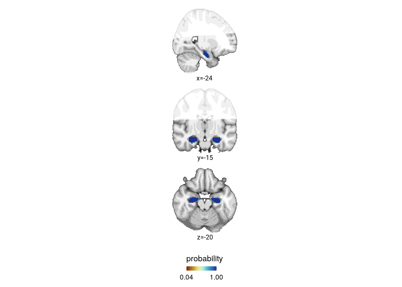
# save source data
file.copy(from = roi_fn, to = file.path(dirs$source_dat_dir, "f4a.nii.gz"))
## [1] TRUEAnterior-lateral entorhinal cortex
# load the ROI
roi_fn <- file.path(dirs$data4analysis, "mni1mm_masks", "alEC_lr_group_prob_mni1mm.nii.gz")
roi_nii <- readNIfTI2(roi_fn)
roi_nii[roi_nii == 0] <- NA

# choose coordinates (these are chosen manually now)
coords <- mni2vox(c(18,1,-35))

# f6a
# get ggplot object for template as background
ggTemplate<-getggTemplate(col_template=rev(RColorBrewer::brewer.pal(8, 'Greys')),brains=mni_nii,
                          all_brain_and_time_inds_one=TRUE,
                          mar=c(1,2,3), mar_ind=coords, col_ind = c(1,1,1),
                          row_ind=sprintf("%s=%d",c("x","y","z"),vox2mni(coords)), center_coords=TRUE)
                          #row_ind=c(1,2,3), center_coords=TRUE)

# get data frame for the ROI image
roi_df <- getBrainFrame(brains=roi_nii, mar=c(1,2,3),
                      row_ind = sprintf("%s=%d",c("x","y","z"),vox2mni(coords)),
                      #row_ind = c(1,2,3), col_ind = c(1,1,1),
                      mar_ind=coords, mask=NULL, center_coords=TRUE)

label_df <- data.frame(row_ind = sprintf("%s=%d",c("x","y","z"),vox2mni(coords)),
                       label = sprintf("%s=%d",c("x","y","z"),vox2mni(coords)))

f6a <- ggTemplate +
  geom_tile(data=roi_df, aes(x=row,y=col,fill=value))+
  facet_wrap(~row_ind, nrow=1, ncol=3, strip.position = "top", scales = "free") +
  scico::scale_fill_scico(palette = "roma",
                          begin = 0, end=1,
                          name = element_blank(),
                          limits = round(range(roi_df$value), digits=2),
                          breaks = round(range(roi_df$value), digits=2)) +
  theme_cowplot(line_size = NA) +
  theme(strip.background = element_blank(), strip.text.x = element_blank(),
        text = element_text(size=10), axis.text = element_text(size=8),
        legend.key.size = unit(0.015, "npc"),
        legend.position = "left", legend.justification = c(0.5, 0.5),
        aspect.ratio = 1
        )+
  guides(fill = guide_colorbar(
    direction = "vertical",
    title.position = "top",
    title.hjust = 0.5,
    label.position = "right"))+
  xlab(element_blank()) + ylab(element_blank()) +
  coord_cartesian(clip = "off") +
  geom_text(data = label_df, x=c(0,0,0), y=c(-85.82,-72.31,-78.1), aes(label = label),
            size = 8/.pt, family=font2use, vjust=1) +
  # y coords found via command below (to keep text aligned across panels):
  # ggplot_build(f6g)$layout$panel_scales_y[[2]]$range$range[1]-diff(ggplot_build(f6g)$layout$panel_scales_y[[2]]$range$range)/100*3
  theme_no_ticks()
print(f6a)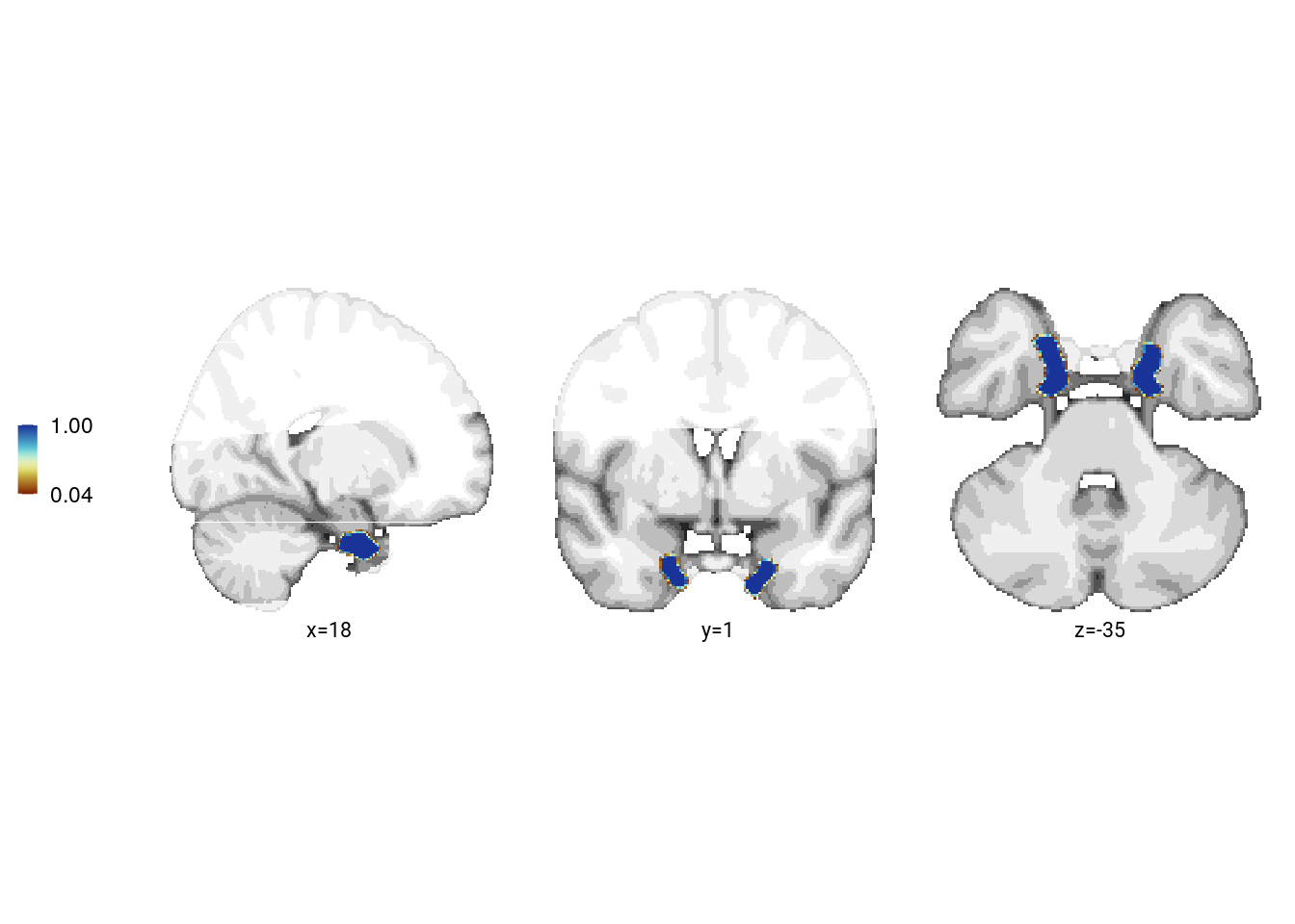
# save source data
file.copy(from = roi_fn, to = file.path(dirs$source_dat_dir, "f6a.nii.gz"))
## [1] TRUE8.3 First-level RSA
In the summary statistics approach, we used the different time metrics as predictors for pattern similarity change. We set up a GLM with the given variable from the day learning task as a predictor and the pairwise representational change values as the criterion for every participant. The t-values of the resulting model coefficients were then compared to a null distribution obtained from shuffling the dependent variable of the linear model (i.e. pattern similarity change) 10,000 times. This approach to permutation-testing of regression coefficients controls Type I errors even under situations of collinear regressors106. Resulting p-values for each coefficient were transformed to a Z-score. The Z-scores were then used for group-level inferential statistics.
Group-level statistics were carried out using permutation-based procedures. For t-tests, we compared the observed t-values against a surrogate distribution obtained from 10,000 random sign-flips to non-parametrically test against 0 or to assess within-participant differences between conditions (two-sided tests; α=0.05 unless stated otherwise). We report Cohen’s d with Hedges’ correction and its 95% confidence interval as computed using the effsize-package for R. For paired tests, Cohen’s d was calculated using pooled standard deviations and confidence intervals are based on the non-central t-distribution. Permutation-based repeated measures ANOVAs were carried out using the permuco-package107 and we report generalized η2 as effect sizes computed using the afex-package(108).
For the summary statistics approach, let’s run the first-level analysis using virtual time as a predictor of pattern similarity change separately for each participant and each ROI. For simplicity we run these analysis together here and will run separate group-level stats below.
set.seed(100) # set seed for reproducibility

# select the data from alEC and HPC
rsa_dat_mtl <- rsa_dat %>%
  filter(roi == "alEC_lr" | roi == "aHPC_lr")

# do RSA using linear model and calculate z-score for model fit based on permutations
rsa_fit <- rsa_dat_mtl %>% group_by(sub_id, roi, same_day) %>%
          # run the linear model
          do(z = lm_perm_jb(in_dat = ., lm_formula = "ps_change ~ vir_time_diff", nsim = n_perm)) %>%
  mutate(z = list(setNames(z, c("z_intercept", "z_virtual_time")))) %>%
  unnest_wider(z)

# add group column used for plotting
rsa_fit$group <- factor(1)

# add a factor with character labels for within/across days and one to later color control in facets
rsa_fit <- rsa_fit %>%
  mutate(same_day_char = plyr::mapvalues(same_day,
                                         from = c(0, 1),
                                         to = c("across days", "within days"),
                                         warn_missing = FALSE),
         same_day_char = factor(same_day_char, levels = c("within days", "across days"))) %>%
  unite(roi_same_day, c("roi", "same_day_char"), remove = FALSE, sep = " ") %>%
  mutate(roi_same_day = str_replace(roi_same_day, "_lr", ":"),
         roi_same_day = factor(roi_same_day, levels = c("aHPC: within days", "aHPC: across days",
                                                        "alEC: within days", "alEC: across days"))
         )
8.4 aHPC: virtual time within sequence
We first test, whether virtual time explains pattern similarity change within the aHPC for event pairs from the same sequence.
Summary statistics
set.seed(101) # set seed for reproducibility

# run a group-level t-test on the RSA fits from the first level in aHPC for within-day
stats <- rsa_fit %>%
  filter(roi == "aHPC_lr", same_day == TRUE) %>%
  select(z_virtual_time) %>%
  paired_t_perm_jb (., n_perm = n_perm)

# Cohen's d with Hedges' correction for one sample using non-central t-distribution for CI
d<-cohen.d(d=(rsa_fit %>% filter(roi == "aHPC_lr", same_day == TRUE))$z_virtual_time, f=NA, paired=TRUE, hedges.correction=TRUE, noncentral=TRUE)
stats$d <- d$estimate
stats$dCI_low <- d$conf.int[[1]]
stats$dCI_high <- d$conf.int[[2]]

# print results
huxtable(stats) %>% theme_article()| estimate | statistic | p.value | p_perm | parameter | conf.low | conf.high | method | alternative | d | dCI_low | dCI_high |
|---|---|---|---|---|---|---|---|---|---|---|---|
| 0.618 | 3.07 | 0.0048 | 0.006 | 27 | 0.205 | 1.03 | One Sample t-test | two.sided | 0.564 | 0.178 | 0.995 |
Summary Statistics: t-test against 0 for virtual time within sequence in aHPC
t27=3.07, p=0.006, d=0.56, 95% CI [0.18, 1.00]
# select the data to plot
plot_dat <- rsa_fit %>% filter(roi == "aHPC_lr", same_day == TRUE)

# raincloud plot
f4b <- ggplot(plot_dat, aes(x=1, y=z_virtual_time, fill = roi, color = roi)) +
  gghalves::geom_half_violin(position=position_nudge(-0.1),
                             side = "l", color = NA) +
  geom_point(aes(x = 1.2, y = z_virtual_time), alpha = 0.7,
             position = position_jitter(width = .1, height = 0),
             shape=16, size = 1) +
  geom_boxplot(position = position_nudge(x = 0, y = 0),
               width = .1, colour = "black", outlier.shape = NA) +
  stat_summary(fun = mean, geom = "point", size = 1, shape = 16,
               position = position_nudge(-0.1), colour = "black") +
  stat_summary(fun.data = mean_se, geom = "errorbar",
               position = position_nudge(-0.1), colour = "black", width = 0, size = 0.5)+
  scale_color_manual(values=unname(aHPC_colors["within_main"])) +
  scale_fill_manual(values=unname(aHPC_colors["within_main"])) +
  ylab('z RSA model fit') + xlab("virtual time") +
  guides(fill = "none", color = "none") +
  annotate(geom = "text", x = 1, y = Inf, label = "**", hjust = 0.5, vjust=1, size = 8/.pt, family=font2use) +
  theme_cowplot() +
  theme(text = element_text(size=10), axis.text = element_text(size=8),
        legend.position = "none",
        axis.ticks.x = element_blank(), axis.text.x = element_blank())
f4b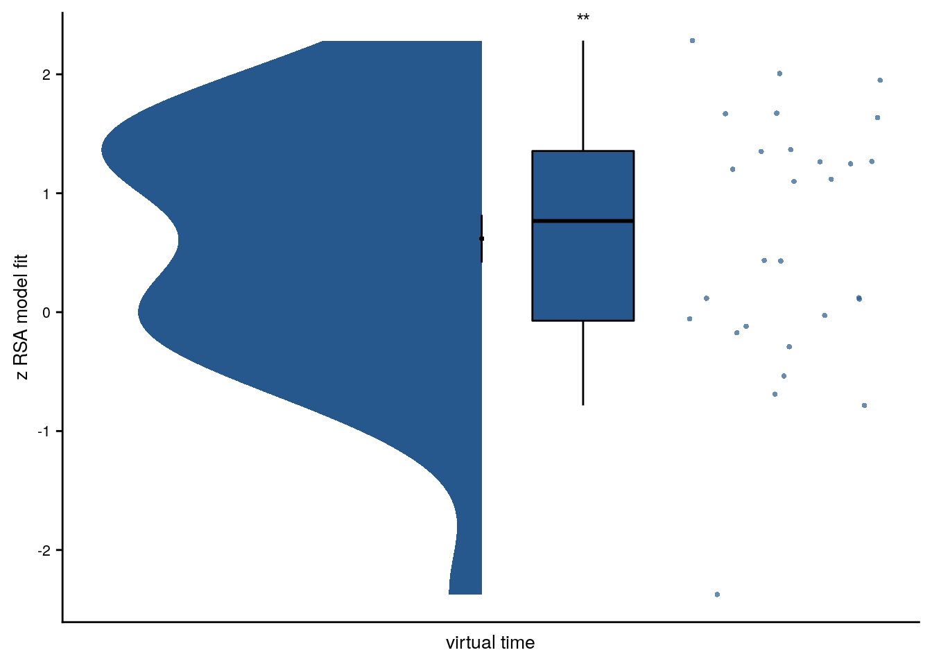
# save source data
source_dat <-ggplot_build(f4b)$data[[2]]
readr::write_tsv(source_dat %>% select(x,y),
                 file = file.path(dirs$source_dat_dir, "f4b.txt"))
Linear Mixed Effects
Likewise, we want to test whether similarity change reflects virtual time differences between elements within a sequence using a mized model. Thus, we use virtual time differences between scenes as the only fixed effect. Following the recommendation for maximal random effect structures by Barr et al. (JML, 2013), we first include random intercepts and random slopes for each subject. This results in a singular fit (random intercept variance estimated as 0). To avoid anti-conservativity we thus drop the correlation between random intercepts and random slopes as suggested by Barr et al., who demonstrate that “LMEMs with maximal random slopes, but missing either random correlations or within-unit random intercepts, performed nearly as well as “fully” maximal LMEMs, with the exception of the case where p-values were determined by MCMC sampling” (p. 267). This model converges without warnings. Below are the model summaries.
set.seed(56) # set seed for reproducibility

# extract the comparisons from the same day
rsa_dat_same_day <- rsa_dat %>%
  filter(roi == "aHPC_lr", same_day == TRUE)

# define the full model with virtual time difference as
# fixed effect and random intercepts for subject
# maximal random effects structure with random slopes and intercepts --> singular fit
formula <- "ps_change ~ vir_time_diff + (1 + vir_time_diff | sub_id)"
lmm_full <- lme4::lmer(formula, data = rsa_dat_same_day, REML = FALSE, control=lmerControl(optCtrl=list(maxfun=20000)))
## boundary (singular) fit: see ?isSingular# thus we reduce the random effects structure. Following Barr et al. (2013), we drop the correlation between random intercepts and random slopes
set.seed(345) # set seed for reproducibility
formula <- "ps_change ~ vir_time_diff + (1 + vir_time_diff || sub_id)"
lmm_full <- lme4::lmer(formula, data = rsa_dat_same_day, REML = FALSE, control=lmerControl(optCtrl=list(maxfun=20000)))
summary(lmm_full, corr = FALSE)## Linear mixed model fit by maximum likelihood ['lmerMod']
## Formula: ps_change ~ vir_time_diff + ((1 | sub_id) + (0 + vir_time_diff | sub_id))
## Data: rsa_dat_same_day
## Control: lmerControl(optCtrl = list(maxfun = 20000))
##
## AIC BIC logLik deviance df.resid
## -7951.4 -7926.3 3980.7 -7961.4 1115
##
## Scaled residuals:
## Min 1Q Median 3Q Max
## -3.4983 -0.6232 -0.0284 0.6645 3.8269
##
## Random effects:
## Groups Name Variance Std.Dev.
## sub_id (Intercept) 6.434e-13 8.021e-07
## sub_id.1 vir_time_diff 6.598e-08 2.569e-04
## Residual 4.784e-05 6.917e-03
## Number of obs: 1120, groups: sub_id, 28
##
## Fixed effects:
## Estimate Std. Error t value
## (Intercept) -0.0003261 0.0002112 -1.544
## vir_time_diff 0.0007513 0.0002197 3.420# tidy summary of the fixed effects that calculates 95% CIs
lmm_full_bm <- broom.mixed::tidy(lmm_full, effects = "fixed", conf.int=TRUE, conf.method="profile")## Computing profile confidence intervals ...# tidy summary of the random effects
lmm_full_bm_re <- broom.mixed::tidy(lmm_full, effects = "ran_pars")We assess the statistical significance of the fixed effect of virtual time using a likelihood ratio test against a reduced (nested) model that does not have this fixed effect.
# one way of testing for significance is by comparing the likelihood against a simpler model.
# Here, we drop the effect of virtual time difference and run an ANOVA. See e.g. Bodo Winter tutorial
set.seed(348) # set seed for reproducibility
formula <- "ps_change ~ 1 + (1 + vir_time_diff || sub_id)"
lmm_no_vir_time <- lme4::lmer(formula, data = rsa_dat_same_day, REML = FALSE)## boundary (singular) fit: see ?isSingularlmm_aov <- anova(lmm_no_vir_time, lmm_full)
lmm_aov| npar | AIC | BIC | logLik | deviance | Chisq | Df | Pr(>Chisq) |
|---|---|---|---|---|---|---|---|
| 4 | -7.94e+03 | -7.92e+03 | 3.98e+03 | -7.95e+03 | |||
| 5 | -7.95e+03 | -7.93e+03 | 3.98e+03 | -7.96e+03 | 9.87 | 1 | 0.00168 |
Mixed Model: Fixed effect of virtual time on aHPC pattern similarity change \(\chi^2\)(1)=9.87, p=0.002
Make mixed model summary table that includes overview of fixed and random effects as well as the model comparison to the nested (reduced) model.
fe_names <- c("intercept", "virtual time")
re_groups <- c(rep("participant",2), "residual")
re_names <- c("intercept (SD)", "virtual time", "SD")
lmm_hux <- make_lme_huxtable(fix_df=lmm_full_bm,
ran_df = lmm_full_bm_re,
aov_mdl = lmm_aov,
fe_terms =fe_names,
re_terms = re_names,
re_groups = re_groups,
lme_form = gsub(" ", "", paste0(deparse(formula(lmm_full)),
collapse = "", sep="")),
caption = "Mixed Model: Virtual time explains representational change for same-sequence events in the anterior hippocampus")
# convert the huxtable to a flextable for word export
stable_lme_aHPC_virtime_same_seq <- convert_huxtable_to_flextable(ht = lmm_hux)
# print to screen
theme_article(lmm_hux)| fixed effects | ||||||
|---|---|---|---|---|---|---|
| term | estimate | SE | t-value | 95% CI | ||
| intercept | -0.000326 | 0.000211 | -1.54 | -0.000740 | 0.000088 | |
| virtual time | 0.000751 | 0.000220 | 3.42 | 0.000307 | 0.001196 | |
| random effects | ||||||
| group | term | estimate | ||||
| participant | intercept (SD) | 0.000001 | ||||
| participant | virtual time | 0.000257 | ||||
| residual | SD | 0.006917 | ||||
| model comparison | ||||||
| model | npar | AIC | LL | X2 | df | p |
| reduced model | 4 | -7943.56 | 3975.78 | |||
| full model | 5 | -7951.43 | 3980.72 | 9.87 | 1 | 0.002 |
| model: ps_change~vir_time_diff+((1|sub_id)+(0+vir_time_diff|sub_id)); SE: standard error, CI: confidence interval, SD: standard deviation, npar: number of parameters, LL: log likelihood, df: degrees of freedom, corr.: correlation | ||||||
lmm_full_bm <- lmm_full_bm %>%
mutate(term=as.factor(term))
# dot plot of Fixed Effect Coefficients with CIs
sfigmm_c <- ggplot(data = lmm_full_bm[2,], aes(x = term, color = term)) +
geom_hline(yintercept = 0, colour="black", linetype="dotted") +
geom_errorbar(aes(ymin = conf.low, ymax = conf.high, width = NA), size = 0.5) +
geom_point(aes(y = estimate), shape = 16, size = 1) +
scale_fill_manual(values = unname(aHPC_colors["within_main"])) +
scale_color_manual(values = unname(aHPC_colors["within_main"]), labels = c("virtual time (same seq)")) +
scale_y_continuous(breaks = seq(from=0, to=0.00125, by=0.00025),
labels = c("0.000", "", "", "", 0.001, "")) +
labs(x = "virtual time", y="fixed effect\ncoefficient", color = "Time Metric") +
guides(color = "none") +
annotate(geom = "text", x = 1, y = Inf, label = "**", hjust = 0.5, vjust=1, size = 8/.pt, family=font2use) +
theme_cowplot() +
theme(plot.title = element_text(hjust = 0.5), axis.text.x=element_blank())
sfigmm_c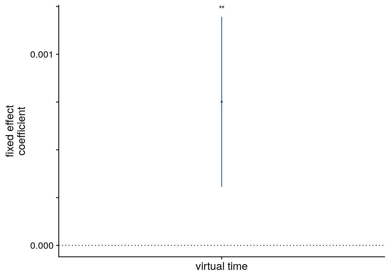
# estimate marginal means for each model term by omitting the terms argument
lmm_full_emm <- ggeffects::ggpredict(lmm_full, ci.lvl = 0.95) %>% get_complete_df()
# plot marginal means
sfigmm_d <- ggplot(data = lmm_full_emm, aes(color = group)) +
geom_line(aes(x, predicted)) +
geom_ribbon(aes(x, ymin = conf.low, ymax = conf.high, fill = group), alpha = .2, linetype=0) +
scale_color_manual(values = unname(aHPC_colors["within_main"])) +
scale_fill_manual(values = unname(aHPC_colors["within_main"])) +
ylab('estimated\nmarginal means') +
xlab('z virtual time') +
guides(color = "none", fill = "none") +
theme_cowplot()
sfigmm_d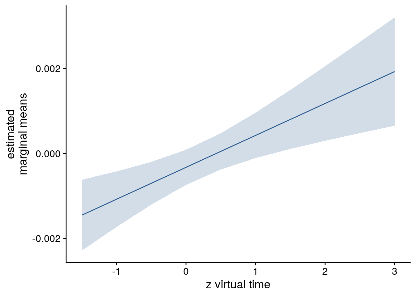
LME model assumptions
lmm_diagplots_jb(lmm_full)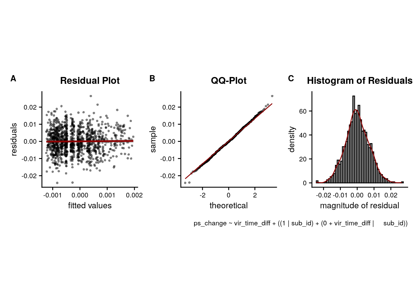
Representational Change Visualization
To illustrate the effect in a simpler way, we average pattern similarity changes based on a median split of events, separately for events from the same and from different sequences.
# get data from aHPC
rsa_dat_hpc <- rsa_dat %>%
filter(roi == "aHPC_lr")
# for each subject, ROI and same/diff day comparisons dichotomize virtual time difference
# based on a median split, then average high/low temporal distances
ps_change_means <-rsa_dat_hpc %>% group_by(sub_id, same_day) %>%
mutate(temp_dist = sjmisc::dicho(vir_time_diff, as.num = TRUE)+1) %>%
group_by(sub_id, same_day, temp_dist) %>%
summarise(ps_change = mean(ps_change), .groups = 'drop')
# make the high/low temporal distance variable a factor
ps_change_means <- ps_change_means %>%
mutate(
temp_dist = as.numeric(temp_dist),
temp_dist_f = factor(temp_dist),
temp_dist_f = plyr::mapvalues(temp_dist, from = c(1,2), to = c("low", "high")),
temp_dist_f = factor(temp_dist_f, levels= c("low", "high")),
same_day = as.factor(same_day),
same_day = plyr::mapvalues(same_day, from = c("FALSE", "TRUE"), to = c("different day", "same day")),
same_day = factor(same_day, levels = c("same day", "different day")))
# Test pattern similarity for same-sequence events separated by high vs. low temporal distances
set.seed(208) # set seed for reproducibility
stats_same_day_high_low <- paired_t_perm_jb(ps_change_means[ps_change_means$same_day=="same day" & ps_change_means$temp_dist_f == "high",]$ps_change -
ps_change_means[ps_change_means$same_day=="same day" & ps_change_means$temp_dist_f == "low",]$ps_change)
# Cohen's d with Hedges' correction for paired samples using non-central t-distribution for CI
d<-cohen.d(d=ps_change_means[ps_change_means$same_day=="same day" & ps_change_means$temp_dist_f == "high",]$ps_change,
f=ps_change_means[ps_change_means$same_day=="same day" & ps_change_means$temp_dist_f == "low",]$ps_change,
paired=TRUE, pooled=TRUE, hedges.correction=TRUE, noncentral=TRUE)
stats_same_day_high_low$d <- d$estimate
stats_same_day_high_low$dCI_low <- d$conf.int[[1]]
stats_same_day_high_low$dCI_high <- d$conf.int[[2]]
huxtable(stats_same_day_high_low) %>% theme_article()| estimate | statistic | p.value | p_perm | parameter | conf.low | conf.high | method | alternative | d | dCI_low | dCI_high |
|---|---|---|---|---|---|---|---|---|---|---|---|
| 0.001 | 2.48 | 0.0197 | 0.0201 | 27 | 0.000173 | 0.00183 | One Sample t-test | two.sided | 0.637 | 0.0752 | 0.871 |
To visualize the effect, lets make a plot of the raw pattern similarity change for high vs. low temporal distances.
# add a column with subject-specific jitter
# generate custom repeating jitter (multiply with -1/1 to shift towards each other)
ps_change_means <- ps_change_means %>%
mutate(
x_jit = as.numeric(temp_dist) + rep(jitter(rep(0,n_subs), amount = 0.05), each=4) * rep(c(-1,1),n_subs))
f4c <- ggplot(data=ps_change_means %>% filter(same_day == "same day"), aes(x=temp_dist, y=ps_change, fill = same_day, color = same_day)) +
gghalves::geom_half_violin(data = ps_change_means %>% filter(same_day == "same day", temp_dist_f == "low"),
aes(x=temp_dist, y=ps_change),
position=position_nudge(-0.1),
side = "l", color = NA) +
gghalves::geom_half_violin(data = ps_change_means %>% filter(same_day == "same day", temp_dist_f == "high"),
aes(x=temp_dist, y=ps_change),
position=position_nudge(0.1),
side = "r", color = NA) +
geom_boxplot(aes(group = temp_dist),width = .1, colour = "black", outlier.shape = NA) +
geom_line(aes(x = x_jit, group=sub_id,), color = ultimate_gray,
position = position_nudge(c(0.15, -0.15))) +
geom_point(aes(x=x_jit), position = position_nudge(c(0.15, -0.15)),
shape=16, size = 1) +
stat_summary(fun = mean, geom = "point", size = 1, shape = 16,
position = position_nudge(c(-0.1, 0.1)), colour = "black") +
stat_summary(fun.data = mean_se, geom = "errorbar",
position = position_nudge(c(-0.1, 0.1)), colour = "black", width = 0, size = 0.5) +
scale_fill_manual(values = unname(aHPC_colors["within_main"])) +
scale_color_manual(values = unname(aHPC_colors["within_main"]), name = "same sequence", labels = "virtual time") +
scale_x_continuous(breaks = c(1,2), labels=c("low", "high")) +
annotate(geom = "text", x = 1.5, y = Inf, label = 'underline(" * ")',
hjust = 0.5, vjust=1, size = 8/.pt, family=font2use, parse=TRUE) +
ylab('pattern similarity change') + xlab('virtual temporal distance') +
guides(fill= "none", color=guide_legend(override.aes=list(fill=NA, alpha = 1, size=2), title.position = "left")) +
theme_cowplot() +
theme(text = element_text(size=10), axis.text = element_text(size=8),
legend.position = "right", strip.background = element_blank(), strip.text = element_blank())
# save source data
source_dat <-ggplot_build(f4c)$data[[4]]
readr::write_tsv(source_dat %>% select(x,y, group),
file = file.path(dirs$source_dat_dir, "f4c.txt"))Summary Statistics: paired t-test for aHPC pattern similarity changes for high vs. low temporal distances for same sequence events t27=2.48, p=0.020, d=0.64, 95% CI [0.08, 0.87]
Not driven by first & last event pairs
In contrast to our previous work(21), where we observed negative correlations of pattern similarity and temporal distances, participants learned multiple sequences in this study. They might have formed strong associations of same-sequence events on top of inferring each event’s virtual time, potentially altering how temporal distances affected hippocampal pattern similarity (see Discussion). The effect of virtual temporal distances on pattern similarity changes remained significant when competing for variance with a control predictor accounting for comparisons of the first and last event of each sequence (Supplemental Figure 5A-C; summary statistics: t27=2.25, p=0.034, d=0.41, 95%% CI [0.04, 0.82]; mixed model: χ2(1)=5.36, p=0.021, Supplemental Table 3). Thus, the relationship of hippocampal event representations and temporal distances is not exclusively driven by associations of the events marking the transitions between sequences.
Now, let’s see if the within-day hippocampus effect goes beyond the effect of the most extreme comparisons, i.e. comparisons between the first and last day of an event. These could for example be used by participants to chunk the events into virtual days. For that we create a binary variable (deviation-coded) that tells us whether a comparison is between the first and last event of a virtual day.
Summary Statistics
In the summary statistics approach, let’s test a multiple regression model that includes the virtual time predictor and a binary predictor for those first/last event pairs. The code below implements the first- and second-level analysis.
set.seed(57) # set seed for reproducibility
# extract all comparisons from the same day
rsa_dat_same_day_aHPC <- rsa_dat %>%
filter(roi == "aHPC_lr", same_day == TRUE)
# find comparisons of first and last event, which are the comparisons of events 1 and 5
# that have an order difference of 4
rsa_dat_same_day_aHPC$first_last <- abs(rsa_dat_same_day_aHPC$event1 - rsa_dat_same_day_aHPC$event2) == 4
# do RSA using linear model and calculate z-score for model fit from permutations
rsa_fit_aHPC_first_last <- rsa_dat_same_day_aHPC %>% group_by(sub_id) %>%
# run the linear model
do(z = lm_perm_jb(in_dat = .,
lm_formula = "ps_change ~ vir_time_diff + first_last",
nsim = n_perm)) %>%
mutate(z = list(setNames(z, c("z_intercept", "z_virtual_time", "z_first_last")))) %>%
unnest_longer(z) %>%
filter(z_id != "z_intercept")
# run group-level t-tests on the RSA fits from the first level in aHPC for within-day
stats <- rsa_fit_aHPC_first_last %>%
filter(z_id == "z_virtual_time") %>%
select(z) %>%
paired_t_perm_jb (., n_perm = n_perm)
# Cohen's d with Hedges' correction for one sample using non-central t-distribution for CI
d<-cohen.d(d=(rsa_fit_aHPC_first_last %>% filter(z_id=="z_virtual_time"))$z, f=NA, paired=TRUE, hedges.correction=TRUE, noncentral=TRUE)
stats$d <- d$estimate
stats$dCI_low <- d$conf.int[[1]]
stats$dCI_high <- d$conf.int[[2]]
# print results
huxtable(stats) %>% theme_article()| estimate | statistic | p.value | p_perm | parameter | conf.low | conf.high | method | alternative | d | dCI_low | dCI_high |
|---|---|---|---|---|---|---|---|---|---|---|---|
| 0.424 | 2.25 | 0.0327 | 0.0341 | 27 | 0.0375 | 0.811 | One Sample t-test | two.sided | 0.413 | 0.0352 | 0.824 |
Summary Statistics: t-test against 0 for virtual time within sequence in aHPC with first-last-event-pair control predictor in the model
t27=2.25, p=0.034, d=0.41, 95% CI [0.04, 0.82]
# select the data to plot
plot_dat <- rsa_fit_aHPC_first_last %>%
mutate(z_id = factor(z_id, levels = c("z_virtual_time", "z_first_last")))
# raincloud plot
sfiga <- ggplot(plot_dat, aes(x=z_id, y=z, fill = z_id, color = z_id)) +
gghalves::geom_half_violin(position=position_nudge(0.1),
side = "r", color = NA) +
geom_point(aes(x = as.numeric(z_id)-0.2, y = z),
position = position_jitter(width = .1, height = 0),
shape=16, size = 1, alpha = 0.7) +
geom_boxplot(position = position_nudge(x = 0, y = 0),
width = .1, colour = "black", outlier.shape = NA) +
stat_summary(fun = mean, geom = "point", size = 1, shape = 16,
position = position_nudge(.1), colour = "black") +
stat_summary(fun.data = mean_se, geom = "errorbar",
position = position_nudge(.1), colour = "black", width = 0, size = 0.5)+
scale_color_manual(values=unname(c(aHPC_colors["within_main"], ultimate_gray)),
name = "RSA predictor", labels = c("virtual time", "first & last event pair")) +
scale_fill_manual(values=unname(c(aHPC_colors["within_main"], ultimate_gray))) +
scale_x_discrete(labels=c("virtual time", "first & last")) +
ylab('z RSA model fit') + xlab('predictor') +
guides(fill = "none", color = guide_legend(override.aes=list(fill=NA, alpha = 1, size=2))) +
annotate(geom = "text", x = 1, y = Inf, label = "*", hjust = 0.5, vjust = 1, size = 8/.pt, family=font2use) +
theme_cowplot() +
theme(text = element_text(size=10), axis.text = element_text(size=8),
legend.direction = "horizontal", legend.position = "bottom",
legend.justification = "center")
sfiga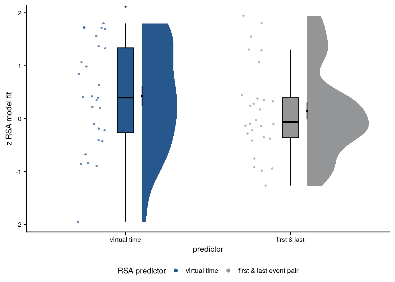
Linear Mixed Effects
Now, let’s do the same using a mixed model. We add the first-last variable as a fixed effect to the model in addition to virtual time to ensure that the effect of virtual time is not exclusively driven by comparisons of the first and last events. The model converges without warnings only with a random effects structure reduced to random slopes for virtual time.
set.seed(58) # set seed for reproducibility
# extract the comparisons from the same day and add variable indicating whether comparison
# is between first and last event of a day
rsa_dat_same_day <- rsa_dat %>% filter(roi == "aHPC_lr", same_day == TRUE) %>%
mutate(first_last = (as.numeric(abs(event1 - event2) == 4)-0.5)*2)
# define the full model with virtual time difference and the extreme pair predictor as
# fixed effects and random intercepts for subject
# maximal random effects structure with random slopes and intercepts --> singular fit
formula <- "ps_change ~ vir_time_diff + first_last + (1 + vir_time_diff + first_last | sub_id)"
lmm_full <- lme4::lmer(formula, data = rsa_dat_same_day, REML = FALSE,
control=lmerControl(optCtrl=list(maxfun=20000)))## boundary (singular) fit: see ?isSingular# thus we remove random intercepts for first-last control predictor -> still singular
set.seed(349) # set seed for reproducibility
formula <- "ps_change ~ vir_time_diff + first_last + (1 + vir_time_diff | sub_id)"
lmm_full <- lme4::lmer(formula, data = rsa_dat_same_day, REML = FALSE,
control=lmerControl(optCtrl=list(maxfun=90000)))## boundary (singular) fit: see ?isSingular# thus we also remove the correlation between random slopes for virtual time and random intercepts
set.seed(349) # set seed for reproducibility
formula <- "ps_change ~ vir_time_diff + first_last + (1 + vir_time_diff || sub_id)"
lmm_full <- lme4::lmer(formula, data = rsa_dat_same_day, REML = FALSE,
control=lmerControl(optCtrl=list(maxfun=90000)))
summary(lmm_full, corr = FALSE)## Linear mixed model fit by maximum likelihood ['lmerMod']
## Formula: ps_change ~ vir_time_diff + first_last + ((1 | sub_id) + (0 + vir_time_diff | sub_id))
## Data: rsa_dat_same_day
## Control: lmerControl(optCtrl = list(maxfun = 90000))
##
## AIC BIC logLik deviance df.resid
## -7950.2 -7920.0 3981.1 -7962.2 1114
##
## Scaled residuals:
## Min 1Q Median 3Q Max
## -3.5046 -0.6260 -0.0376 0.6554 3.8528
##
## Random effects:
## Groups Name Variance Std.Dev.
## sub_id (Intercept) 7.365e-13 8.582e-07
## sub_id.1 vir_time_diff 6.680e-08 2.585e-04
## Residual 4.781e-05 6.914e-03
## Number of obs: 1120, groups: sub_id, 28
##
## Fixed effects:
## Estimate Std. Error t value
## (Intercept) -1.523e-05 4.207e-04 -0.036
## vir_time_diff 6.257e-04 2.644e-04 2.367
## first_last 3.568e-04 4.177e-04 0.854# tidy summary of the fixed effects that calculates 95% CIs
lmm_full_bm <- broom.mixed::tidy(lmm_full, effects = "fixed", conf.int=TRUE, conf.method="profile")## Computing profile confidence intervals ...# tidy summary of the random effects
lmm_full_bm_re <- broom.mixed::tidy(lmm_full, effects = "ran_pars")
# compare against a reduced model
set.seed(301) # set seed for reproducibility
formula <- "ps_change ~ first_last + (1 + vir_time_diff || sub_id)"
lmm_no_vir_time <- lme4::lmer(formula, data = rsa_dat_same_day, REML = FALSE)## boundary (singular) fit: see ?isSingularlmm_aov <- anova(lmm_no_vir_time, lmm_full)Mixed Model: Fixed effect of virtual time on aHPC pattern similarity change with first-last-event-pair control predictor
\(\chi^2\)(1)=5.36, p=0.021
Make mixed model summary table that includes overview of fixed and random effects as well as the model comparison to the nested (reduced) model.
fe_names <- c("intercept", "virtual time", "first-last pair")
re_groups <- c(rep("participant",2), "residual")
re_names <- c("intercept (SD)", "virtual time (SD)", "SD")
lmm_hux <- make_lme_huxtable(fix_df=lmm_full_bm,
ran_df = lmm_full_bm_re,
aov_mdl = lmm_aov,
fe_terms =fe_names,
re_terms = re_names,
re_groups = re_groups,
lme_form = gsub(" ", "", paste0(deparse(formula(lmm_full)),
collapse = "", sep="")),
caption = "Mixed Model: Virtual time explains representational change for same-sequence events in the anterior hippocampus when controlling for the effect of first-last event pairs")
# convert the huxtable to a flextable for word export
stable_lme_aHPC_virtime_same_seq_first_last <- convert_huxtable_to_flextable(ht = lmm_hux)
# print to screen
theme_article(lmm_hux)| fixed effects | ||||||
|---|---|---|---|---|---|---|
| term | estimate | SE | t-value | 95% CI | ||
| intercept | -0.000015 | 0.000421 | -0.04 | -0.000841 | 0.000810 | |
| virtual time | 0.000626 | 0.000264 | 2.37 | 0.000099 | 0.001152 | |
| first-last pair | 0.000357 | 0.000418 | 0.85 | -0.000462 | 0.001176 | |
| random effects | ||||||
| group | term | estimate | ||||
| participant | intercept (SD) | 0.000001 | ||||
| participant | virtual time (SD) | 0.000258 | ||||
| residual | SD | 0.006914 | ||||
| model comparison | ||||||
| model | npar | AIC | LL | X2 | df | p |
| reduced model | 5 | -7946.81 | 3978.40 | |||
| full model | 6 | -7950.16 | 3981.08 | 5.36 | 1 | 0.021 |
| model: ps_change~vir_time_diff+first_last+((1|sub_id)+(0+vir_time_diff|sub_id)); SE: standard error, CI: confidence interval, SD: standard deviation, npar: number of parameters, LL: log likelihood, df: degrees of freedom, corr.: correlation | ||||||
LME Plots.
# let's plot the effect
lmm_full_bm <- lmm_full_bm %>%
mutate(term=factor(term, levels = c("vir_time_diff", "first_last", "(Intercept)")))
# dot plot of Fixed Effect Coefficients with CIs
sfigb <- ggplot(data = lmm_full_bm[c(2,3),], aes(x = term, color = term)) +
geom_hline(yintercept = 0, colour="black", linetype="dotted") +
geom_errorbar(aes(ymin = conf.low, ymax = conf.high, width = NA), size = 0.5) +
geom_point(aes(y = estimate), size = 1, shape = 16) +
#scale_fill_manual(values = c(unname(aHPC_colors["within_main"]), "gray")) +
scale_color_manual(values = c(unname(aHPC_colors["within_main"]), ultimate_gray), labels = c("Virtual Time", "First-last")) +
labs(x = element_blank(), y = "fixed effect\ncoefficient", color = "Time Metric") +
guides(color = "none", fill = "none") +
annotate(geom = "text", x = 1, y = Inf, label = "*", hjust = 0.5, vjust = 1, size = 8/.pt, family=font2use) +
theme_cowplot() +
#coord_fixed(ratio = 3\\\\) +
theme(legend.position = "none", plot.title = element_text(hjust = 0.5), axis.text.x=element_blank())
sfigb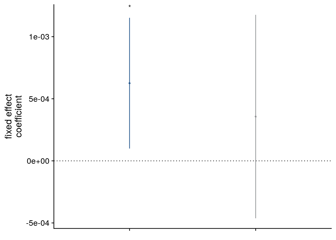
# estimate marginal means for each model term by omitting the terms argument
lmm_full_emm <- ggeffects::ggpredict(lmm_full, ci.lvl = 0.95) %>%
get_complete_df()
# plot marginal means
sfigc <- ggplot(data = lmm_full_emm, aes(color = group)) +
geom_line(aes(x, predicted)) +
geom_ribbon(aes(x, ymin = conf.low, ymax = conf.high, fill = group), alpha = .2, linetype=0,
show.legend = FALSE) +
scale_color_manual(values = c("gray", unname(aHPC_colors["within_main"])),
name = element_blank(), labels =c("first & last event", "virtual time")) +
scale_fill_manual(values = c("gray", unname(aHPC_colors["within_main"]))) +
ylab('estimated\nmarginal means') +
xlab('fixed effect') +
guides(fill = "none", color = "none") +
theme_cowplot()
sfigc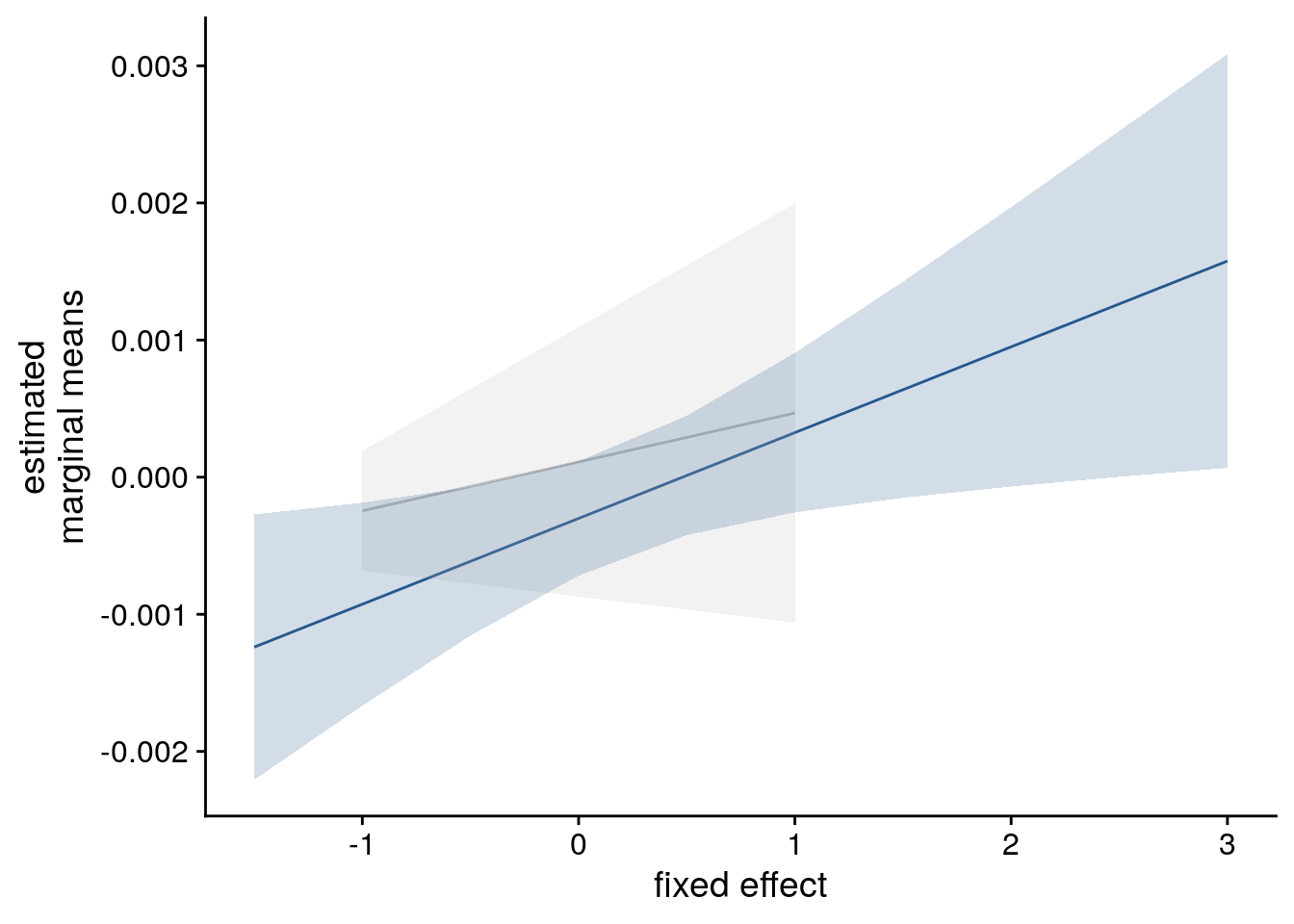
LME model assumptions
lmm_diagplots_jb(lmm_full)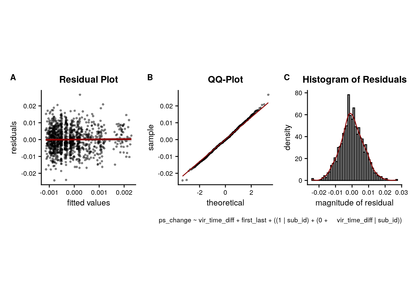
8.5 aHPC: virtual time within sequence when including order & real time
We further tested whether the effect of virtual time on anterior hippocampal pattern similarity change persisted when including the absolute difference between sequence positions (“order”) and the interval in seconds between events (“real time”) as control predictors of no interest in the model.
To follow up on the within-day effect in the hippocampus, let’s see if virtual correlates with pattern similarity change above and beyond the effects of order and real time. We will look at this in two ways.
One model with multiple predictors
The first way is to run models in which the three time metrics compete for variance. Temporal distances based on order and real time are control regressors of no interest, we test only the effect of virtual time for significance.
Summary Statistics
In the summary statistics approach, this comes down to a multiple regression on the participant-level. Again, we compute z-values for each regression coefficient from permutations of the dependent variable, which maintains the correlation structure of the regressors. Then we test the z-values for virtual time against 0 on the group level.
set.seed(59) # set seed for reproducibility
# extract all comparisons from the same day
rsa_dat_same_day_aHPC <- rsa_dat %>%
filter(roi == "aHPC_lr", same_day == TRUE)
# do RSA using linear model and calculate z-score for model fit from permutations
rsa_fit_aHPC_mult_reg <- rsa_dat_same_day_aHPC %>% group_by(sub_id) %>%
# run the linear model
do(z = lm_perm_jb(in_dat = .,
lm_formula = "ps_change ~ vir_time_diff + order_diff + real_time_diff",
nsim = n_perm)) %>%
mutate(z = list(setNames(z, c("z_intercept", "z_virtual_time", "z_order", "z_real_time")))) %>%
unnest_longer(z) %>%
filter(z_id != "z_intercept")
# run group-level t-tests on the RSA fits from the first level in aHPC for within-day
stats <- rsa_fit_aHPC_mult_reg %>%
filter(z_id =="z_virtual_time") %>%
select(z) %>%
paired_t_perm_jb (., n_perm = n_perm)
# Cohen's d with Hedges' correction for one sample using non-central t-distribution for CI
d<-cohen.d(d=(rsa_fit_aHPC_mult_reg %>% filter(z_id == "z_virtual_time"))$z, f=NA, paired=TRUE, hedges.correction=TRUE, noncentral=TRUE)
stats$d <- d$estimate
stats$dCI_low <- d$conf.int[[1]]
stats$dCI_high <- d$conf.int[[2]]
# print results
huxtable(stats) %>% theme_article()| estimate | statistic | p.value | p_perm | parameter | conf.low | conf.high | method | alternative | d | dCI_low | dCI_high |
|---|---|---|---|---|---|---|---|---|---|---|---|
| 0.437 | 2.18 | 0.0385 | 0.0401 | 27 | 0.0248 | 0.849 | One Sample t-test | two.sided | 0.399 | 0.0218 | 0.808 |
Summary Statistics: t-test against 0 for virtual time within sequence in aHPC with order and real time in the model
t27=2.18, p=0.040, d=0.40, 95% CI [0.02, 0.81]
# make z_id a factor and reorder it
rsa_fit_aHPC_mult_reg <- rsa_fit_aHPC_mult_reg %>% mutate(
z_id = factor(z_id, levels = c("z_virtual_time", "z_order", "z_real_time")))
# raincloud plot
f4d <- ggplot(rsa_fit_aHPC_mult_reg, aes(x=z_id, y=z, fill = z_id, colour = z_id)) +
gghalves::geom_half_violin(position=position_nudge(0.1),
side = "r", color = NA) +
geom_point(aes(x = as.numeric(z_id)-0.2), alpha = 0.7,
position = position_jitter(width = .1, height = 0),
shape=16, size = 1) +
geom_boxplot(position = position_nudge(x = 0, y = 0),
width = .1, colour = "black", outlier.shape = NA) +
stat_summary(fun = mean, geom = "point", size = 1, shape = 16,
position = position_nudge(.1), colour = "black") +
stat_summary(fun.data = mean_se, geom = "errorbar",
position = position_nudge(.1), colour = "black", width = 0, size = 0.5)+
ylab('z RSA model fit') + xlab('time metric') +
scale_x_discrete(labels = c("virtual time", "order", "real time")) +
scale_color_manual(values=time_colors, name = "time metric",
labels = c("virtual time", "order", "real time")) +
scale_fill_manual(values=time_colors) +
annotate(geom = "text", x = 1, y = Inf, label = "*", hjust = 0.5, vjust=1, size = 8/.pt, family=font2use) +
guides(fill = "none", color = guide_legend(override.aes=list(fill=NA, alpha = 1, size=2))) +
theme_cowplot() +
theme(text = element_text(size=10), axis.text = element_text(size=8),
legend.position = "none")
f4d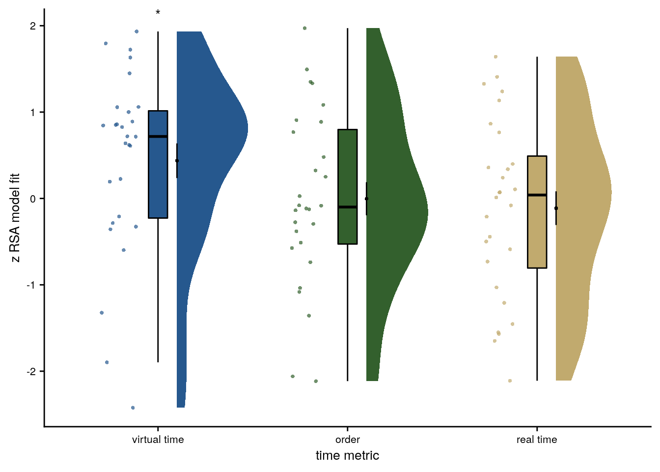
# save source data
source_dat <-ggplot_build(f4d)$data[[2]]
readr::write_tsv(source_dat %>% select(x,y, group),
file = file.path(dirs$source_dat_dir, "f4d.txt"))Linear Mixed Effects
For the mixed model, we use order differences and real time differences as fixed effects in addition to virtual time. As a random effect structure we first include random intercepts and random slopes for each subject for all 3 fixed effects. This model is singular due to an estimated correlation of 1 between random slopes and random intercepts. We remove the random intercepts, but the fit is still singular. Removing the random slopes for the two fixed effects of no interest (order and real time) also does not help. We thus drop the random intercepts (as above) as well to end up with a model that converges without warnings.
Thus, the full model for this analysis has 3 fixed effects and random slopes for virtual time for each subject.
set.seed(87) # set seed for reproducibility
# extract the comparisons from the same day
rsa_dat_same_day <- rsa_dat %>% filter(roi == "aHPC_lr", same_day == TRUE)
# define the full model with virtual time difference, order difference and real time difference as
# fixed effects and random intercepts and random slopes for all effects
# fails to converge and is singular after restart
formula <- "ps_change ~ vir_time_diff + order_diff + real_time_diff + (1+vir_time_diff + order_diff + real_time_diff | sub_id)"
lmm_full <- lme4::lmer(formula, data = rsa_dat_same_day, REML = FALSE)## boundary (singular) fit: see ?isSingular#lmm_full <- update(lmm_full, start=getME(lmm_full, "theta"))
# remove the correlation between random slopes and random intercepts
formula <- "ps_change ~ vir_time_diff + order_diff + real_time_diff + (1+vir_time_diff + order_diff + real_time_diff || sub_id)"
lmm_full <- lme4::lmer(formula, data = rsa_dat_same_day, REML = FALSE)## boundary (singular) fit: see ?isSingular# thus we reduce the random effect structure by excluding random slopes for the fixed effects of no interest
# as above this results in a singular fit (the random intercept variance estimated to be 0)
formula <- "ps_change ~ vir_time_diff + order_diff + real_time_diff + (1+vir_time_diff | sub_id)"
lmm_full <- lme4::lmer(formula, data = rsa_dat_same_day, REML = FALSE)## boundary (singular) fit: see ?isSingular# next step is to remove the correlation between random slopes and random intercepts
formula <- "ps_change ~ vir_time_diff + order_diff + real_time_diff + (1+vir_time_diff || sub_id)"
lmm_full <- lme4::lmer(formula, data = rsa_dat_same_day, REML = FALSE)## boundary (singular) fit: see ?isSingular# we thus reduce further and keep only the random slopes for virtual time differences
# now the model converges without warnings
set.seed(332) # set seed for reproducibility
formula <- "ps_change ~ vir_time_diff + order_diff + real_time_diff + (0 + vir_time_diff | sub_id)"
lmm_full <- lme4::lmer(formula, data = rsa_dat_same_day, REML = FALSE)
summary(lmm_full, corr = FALSE)## Linear mixed model fit by maximum likelihood ['lmerMod']
## Formula: ps_change ~ vir_time_diff + order_diff + real_time_diff + (0 + vir_time_diff | sub_id)
## Data: rsa_dat_same_day
##
## AIC BIC logLik deviance df.resid
## -7950.8 -7920.6 3981.4 -7962.8 1114
##
## Scaled residuals:
## Min 1Q Median 3Q Max
## -3.4923 -0.6444 -0.0269 0.6629 3.8017
##
## Random effects:
## Groups Name Variance Std.Dev.
## sub_id vir_time_diff 6.744e-08 0.0002597
## Residual 4.778e-05 0.0069126
## Number of obs: 1120, groups: sub_id, 28
##
## Fixed effects:
## Estimate Std. Error t value
## (Intercept) -2.812e-04 2.191e-04 -1.284
## vir_time_diff 1.321e-03 5.415e-04 2.439
## order_diff 1.235e-05 9.077e-04 0.014
## real_time_diff -6.760e-04 1.019e-03 -0.663# tidy summary of the fixed effects that calculates 95% CIs
lmm_full_bm <- broom.mixed::tidy(lmm_full, effects = "fixed", conf.int=TRUE, conf.method="profile")## Computing profile confidence intervals ...# tidy summary of the random effects
lmm_full_bm_re <- broom.mixed::tidy(lmm_full, effects = "ran_pars")
# one way of testing for significance is by comparing the likelihood against a simpler model.
# Here, we drop the effect of virtual time difference and run an ANOVA. See e.g. Bodo Winter tutorial
set.seed(321) # set seed for reproducibility
formula <- "ps_change ~ order_diff + real_time_diff + (0 + vir_time_diff | sub_id)"
lmm_no_vir_time <- lme4::lmer(formula, data = rsa_dat_same_day, REML = FALSE)
lmm_aov <- anova(lmm_no_vir_time, lmm_full)
lmm_aov| npar | AIC | BIC | logLik | deviance | Chisq | Df | Pr(>Chisq) |
|---|---|---|---|---|---|---|---|
| 5 | -7.95e+03 | -7.92e+03 | 3.98e+03 | -7.96e+03 | |||
| 6 | -7.95e+03 | -7.92e+03 | 3.98e+03 | -7.96e+03 | 5.92 | 1 | 0.015 |
Mixed Model: Fixed effect of virtual time on aHPC within-sequence pattern similarity change with order and real time in model \(\chi^2\)(1)=5.92, p=0.015
Make mixed model summary table that includes overview of fixed and random effects as well as the model comparison to the nested (reduced) model.
fe_names <- c("intercept", "virtual time", "order", "real time")
re_groups <- c(rep("participant",1), "residual")
re_names <- c("virtual time (SD)", "SD")
lmm_hux <- make_lme_huxtable(fix_df=lmm_full_bm,
ran_df = lmm_full_bm_re,
aov_mdl = lmm_aov,
fe_terms =fe_names,
re_terms = re_names,
re_groups = re_groups,
lme_form = gsub(" ", "", paste0(deparse(formula(lmm_full)),
collapse = "", sep="")),
caption = "Mixed Model: Virtual time explains representational change for same-sequence events in the anterior hippocampus when including order and real time in the model")
# convert the huxtable to a flextable for word export
stable_lme_aHPC_virtime_same_seq_time_metrics <- convert_huxtable_to_flextable(ht = lmm_hux)
# print to screen
theme_article(lmm_hux)| fixed effects | ||||||
|---|---|---|---|---|---|---|
| term | estimate | SE | t-value | 95% CI | ||
| intercept | -0.000281 | 0.000219 | -1.28 | -0.000711 | 0.000149 | |
| virtual time | 0.001321 | 0.000541 | 2.44 | 0.000258 | 0.002383 | |
| order | 0.000012 | 0.000908 | 0.01 | -0.001768 | 0.001793 | |
| real time | -0.000676 | 0.001019 | -0.66 | -0.002675 | 0.001323 | |
| random effects | ||||||
| group | term | estimate | ||||
| participant | virtual time (SD) | 0.000260 | ||||
| residual | SD | 0.006913 | ||||
| model comparison | ||||||
| model | npar | AIC | LL | X2 | df | p |
| reduced model | 5 | -7946.84 | 3978.42 | |||
| full model | 6 | -7950.76 | 3981.38 | 5.92 | 1 | 0.015 |
| model: ps_change~vir_time_diff+order_diff+real_time_diff+(0+vir_time_diff|sub_id); SE: standard error, CI: confidence interval, SD: standard deviation, npar: number of parameters, LL: log likelihood, df: degrees of freedom, corr.: correlation | ||||||
Mixed model plots.
# set RNG
set.seed(23)
lmm_full_bm <- lmm_full_bm %>%
mutate(term=as.factor(term) %>%
factor(levels = c("vir_time_diff", "order_diff", "real_time_diff")))
# dot plot of Fixed Effect Coefficients with CIs
sfigmm_e <- ggplot(data = lmm_full_bm[2:4,], aes(x = term, color = term)) +
geom_hline(yintercept = 0, colour="black", linetype="dotted") +
geom_errorbar(aes(ymin = conf.low, ymax = conf.high, width = NA), size = 0.5) +
geom_point(aes(y = estimate), shape = 16, size = 1) +
scale_fill_manual(values = time_colors) +
scale_color_manual(values = time_colors, labels = c("virtual time (same seq.)", "order", "real Time")) +
labs(x = "time metric", y = "fixed effect\nestimate", color = "Time Metric") +
guides(color = "none", fill = "none") +
annotate(geom = "text", x = 1, y = Inf, label = "*", hjust = 0.5, vjust = 1, size = 8/.pt, family=font2use) +
theme_cowplot() +
theme(plot.title = element_text(hjust = 0.5), axis.text.x=element_blank())
sfigmm_e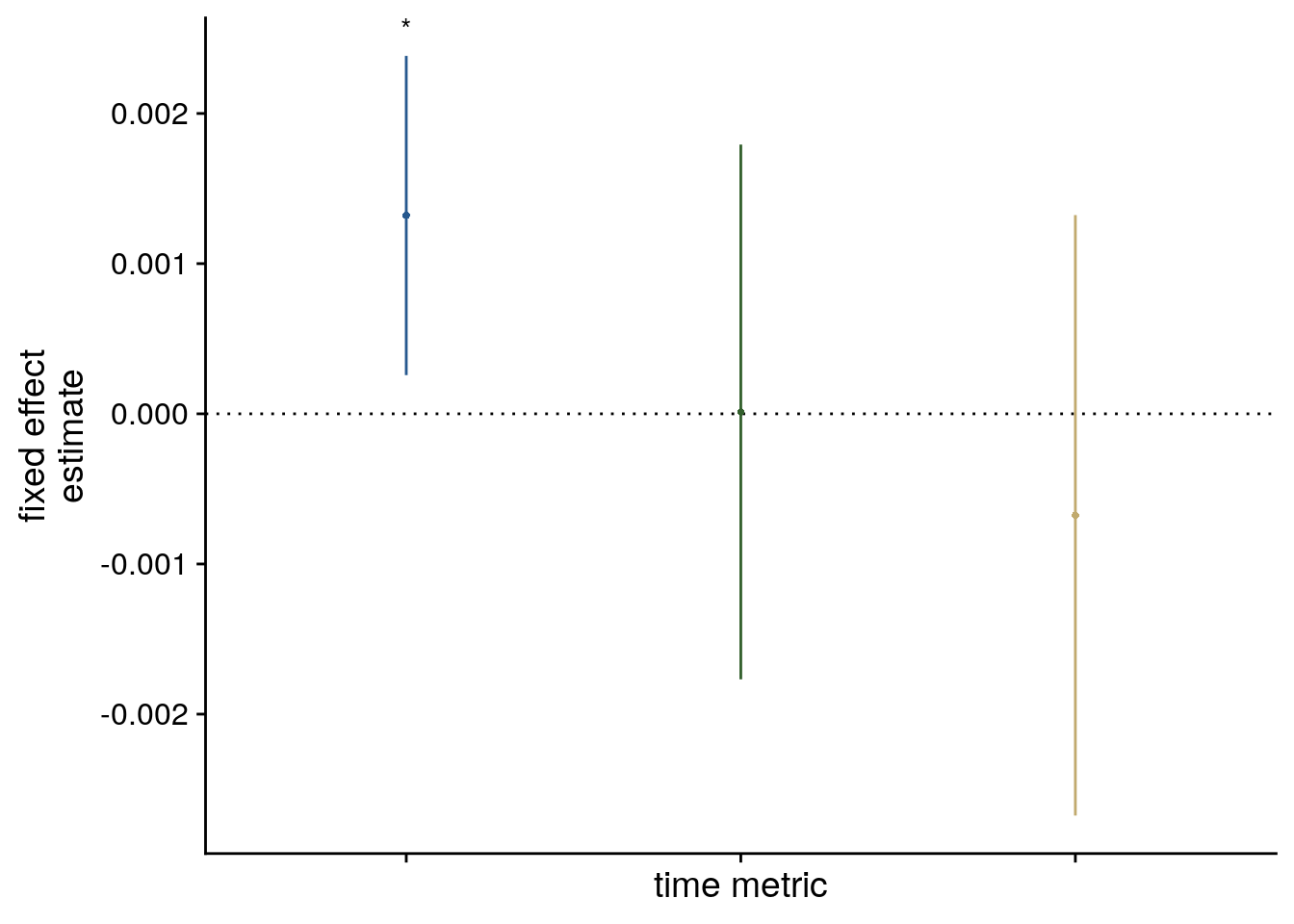
# estimate marginal means for each model term by omitting the terms argument
lmm_full_emm <- ggeffects::ggpredict(lmm_full, ci.lvl = 0.95) %>% get_complete_df
# convert the group variable to a factor to control the order of facets below
lmm_full_emm$group <- factor(lmm_full_emm$group, levels = c("vir_time_diff", "order_diff", "real_time_diff"))
# plot marginal means
sfigmm_f <- ggplot(data = lmm_full_emm, aes(color = group)) +
geom_line(aes(x, predicted)) +
geom_ribbon(aes(x, ymin = conf.low, ymax = conf.high, fill = group), alpha = .2, linetype=0) +
scale_color_manual(values = time_colors, name = element_blank(),
labels = c("virtual time", "order", "real time")) +
scale_fill_manual(values = time_colors) +
ylab('estimated\nmarginal means') +
xlab('z time metric') +
guides(fill = "none", color = "none") +
theme_cowplot() +
theme(plot.title = element_text(hjust = 0.5), strip.background = element_blank(),
strip.text.x = element_blank())
sfigmm_f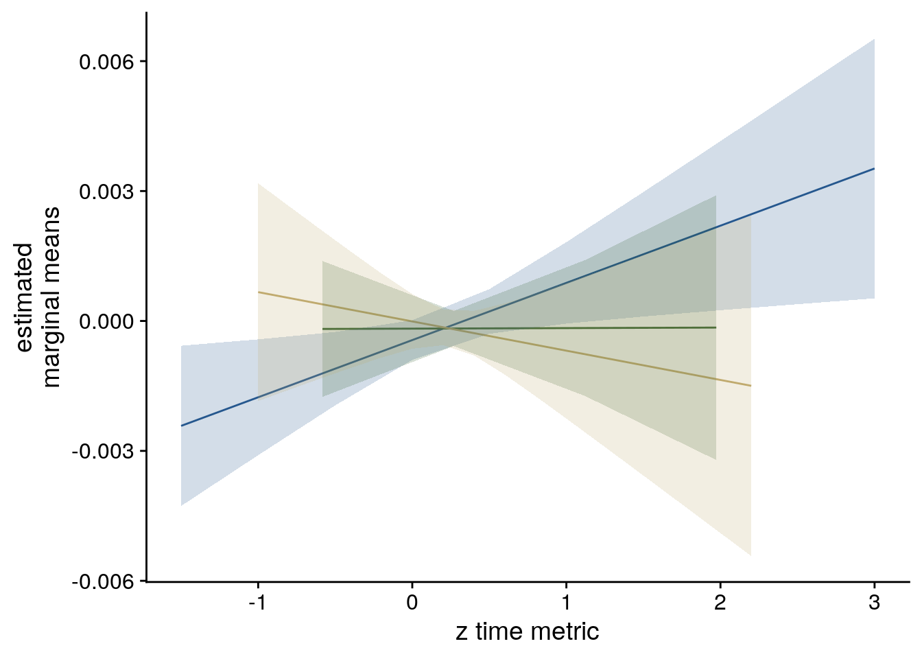
LME model assumptions
lmm_diagplots_jb(lmm_full)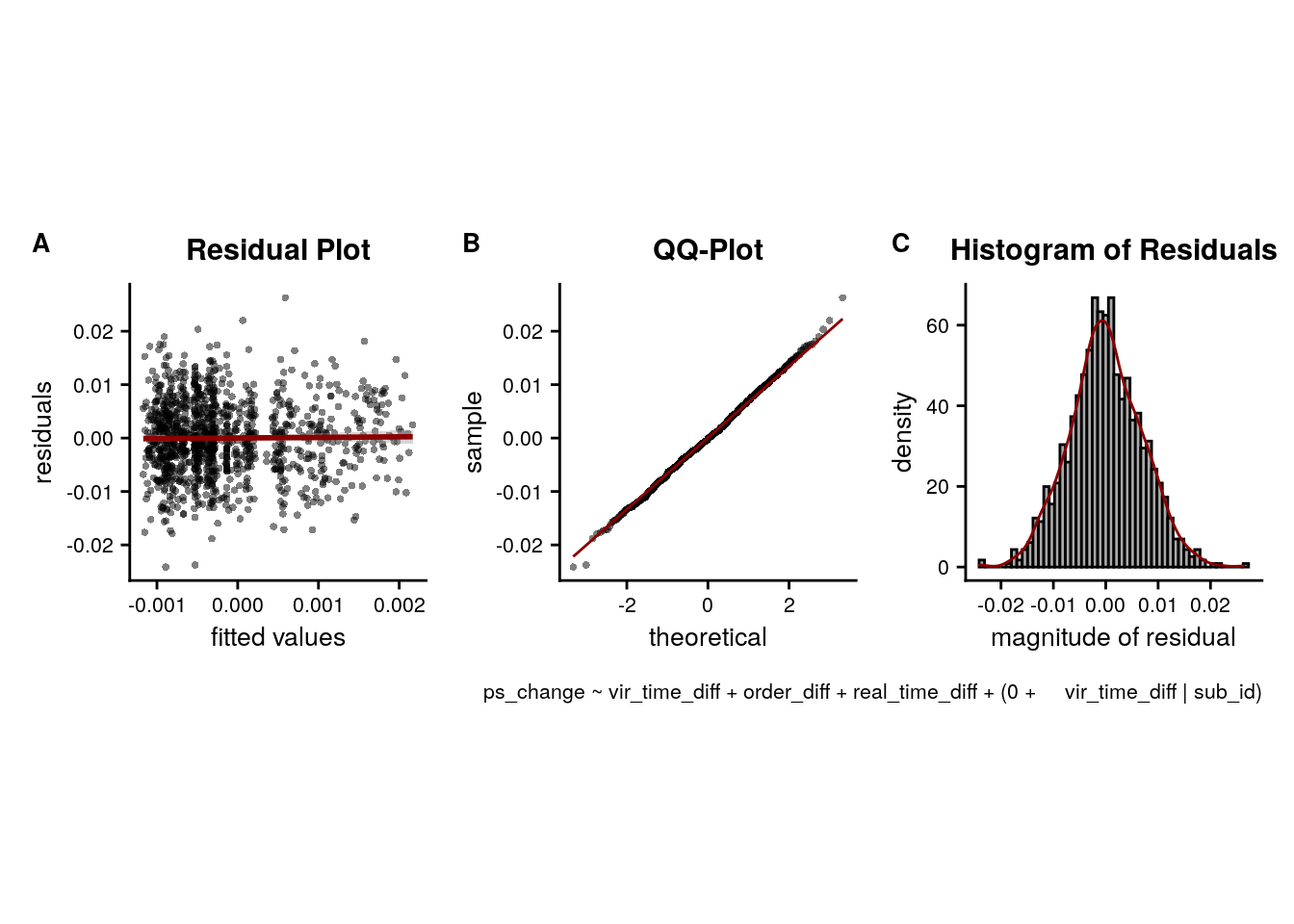
We are now ready to create figure 4 of the manuscript:
layoutBD = "BBCCCDDD"
layoutABD ="
ABBBBBB
ABBBBBB"
f4 <- f4a+
{f4b + f4c + f4d +
plot_layout(design = layoutBD, guides = "collect") &
theme(text = element_text(size=10, family=font2use),
axis.text = element_text(size=8),
legend.text=element_text(size=8),
legend.title=element_text(size=8),
legend.spacing.x = unit(1, 'mm'),
legend.key.size = unit(3,"mm"),
legend.position = 'bottom', legend.justification = "right",
legend.margin = margin(0,0,0,1, unit="cm"))} +
plot_layout(design = layoutABD, guides = "keep") &
plot_annotation(theme = theme(plot.margin = margin(t=0, r=0, b=0, l=-19, unit="pt")),
tag_levels = 'A')&
theme(text = element_text(size=10, family=font2use))
f4[[1]] <- f4[[1]] +
theme(legend.position = c(0.5,-0.1963),
legend.text=element_text(size=8),
legend.title=element_text(size=8),
plot.tag = element_text(margin = margin(l = 13)))
# save and print
fn <- here("figures", "f4")
ggsave(paste0(fn, ".pdf"), plot=f4, units = "cm",
width = 18, height = 10, dpi = "retina", device = cairo_pdf)
ggsave(paste0(fn, ".png"), plot=f4, units = "cm",
width = 18, height = 10, dpi = "retina", device = "png")
Figure 4. Sequence representations in anterior hippocampus reflect constructed event times. A. The anterior hippocampus region of interest is displayed on the MNI template with voxels outside the field of view shown in lighter shades of gray. Color code denotes probability of a voxel to be included in the mask based on participant-specific ROIs (see Methods). B. The Z-values based on permutation tests of participant-specific linear models assessing the effect of virtual time on pattern similarity change for event pairs from the same sequence were significantly positive. C. To illustrate the effect shown in B, average pattern similarity change values are shown for same-sequence event pairs that are separated by low and high temporal distances based on a median split. D. Z-values show the relationship of the different time metrics to representational change based on participant-specific multiple regression analyses. Virtual time predicts pattern similarity change with event order and real time in the model as control predictors of no interest. B-D. Circles are individual participant data; boxplots show median and upper/lower quartile along with whiskers extending to most extreme data point within 1.5 interquartile ranges above/below the upper/lower quartile; black circle with error bars corresponds to mean±S.E.M.; distributions show probability density function of data points. ** p<0.01; * p<0.05
Virtual time explains residuals of order and real time
We implemented participant-specific regression analyses with order and real time distances as predictors of hippocampal pattern similarity change. The plot shows a significant effect of virtual temporal distances when tested on the residuals of these linear models. Thus, variance that cannot be explained by the other time metrics can be accounted for by virtual temporal distances. This analysis was conducted only using the summary statistics approach because the residuals of a mixed model are more difficult to interpret than those of participant-specific regression analyses using ordinary least squares.
The second way of running this analysis is via a two-step procedure. We first predict pattern similarity change from the ordinal and real-time relationships and store the residuals, i.e. variance in pattern similarity change that cannot be explained by the effects of order and real time. Then, we test in a second model whether virtual time can explain these residuals.
Summary Statistics
The first step here is a multiple linear regression model with order and real time distances as predictors. We do not use permutations here because we are only interested in the residuals of this model. In the second step, we run a linear model with permutations to obtain z-values for group-level stats for the effect of virtual time on the residuals.
set.seed(102) # set seed for reproducibility
# extract all comparisons from the same day
rsa_dat_same_day_aHPC <- rsa_dat %>%
filter(roi == "aHPC_lr", same_day == TRUE)
# run multiple regression model with order and real time as predictors and store residuals
resids <- rsa_dat_same_day_aHPC %>% group_by(sub_id) %>%
# run the linear model
do(resids = residuals(lm(ps_change ~ order_diff + real_time_diff, data=.))) %>%
select(resids) %>%
unnest(resids)
# add to the original data frame
rsa_dat_same_day_aHPC$resids <- resids$resids
# do RSA using linear model and calculate z-score for model fit
rsa_fit_aHPC_mult_reg_resids <- rsa_dat_same_day_aHPC %>%
group_by(sub_id) %>%
# run the linear model
do(z = lm_perm_jb(in_dat = .,
lm_formula = "resids ~ vir_time_diff",
nsim = n_perm)) %>%
mutate(z = list(setNames(z, c("z_intercept", "z_virtual_time")))) %>%
unnest_wider(z)
# run a group-level t-test on the RSA fits from the first level in aHPC for within-day
stats <- rsa_fit_aHPC_mult_reg_resids %>%
select(z_virtual_time) %>%
paired_t_perm_jb (., n_perm = n_perm)
# Cohen's d with Hedges' correction for one sample using non-central t-distribution for CI
d<-cohen.d(d=rsa_fit_aHPC_mult_reg_resids$z_virtual_time,
f=NA, paired=TRUE, hedges.correction=TRUE, noncentral=TRUE)
stats$d <- d$estimate
stats$dCI_low <- d$conf.int[[1]]
stats$dCI_high <- d$conf.int[[2]]
# print results
huxtable(stats) %>% theme_article()| estimate | statistic | p.value | p_perm | parameter | conf.low | conf.high | method | alternative | d | dCI_low | dCI_high |
|---|---|---|---|---|---|---|---|---|---|---|---|
| 0.177 | 2.23 | 0.0345 | 0.0343 | 27 | 0.014 | 0.341 | One Sample t-test | two.sided | 0.409 | 0.031 | 0.819 |
Summary Statistics for virtual time on residuals of order and real time:
t27=2.23, p=0.034, d=0.41, 95% CI [0.03, 0.82]
We further observed that the residuals of linear models, in which hippocampal representational change was predicted from order and real time, were related to virtual temporal distances (Supplemental Figure 3D; t27=2.23, p=0.034, d=0.41, 95% CI [0.03, 0.82] ), demonstrating that virtual time accounts for variance that the other time metrics fail to explain.
# select the data to plot
plot_dat <- rsa_fit_aHPC_mult_reg_resids
plot_dat$group <- factor(1)
# raincloud
sfigd <- ggplot(plot_dat, aes(x=1, y=z_virtual_time, color = group, fill=group)) +
gghalves::geom_half_violin(position=position_nudge(0.1),
side = "r", color = NA) +
geom_point(aes(x = 0.8, y = z_virtual_time), alpha = 0.7,
position = position_jitter(width = .1, height = 0),
shape=16, size = 1) +
geom_boxplot(position = position_nudge(x = 0, y = 0),
width = .1, colour = "black", outlier.shape = NA) +
stat_summary(fun = mean, geom = "point", size = 1, shape = 16,
position = position_nudge(.1), colour = "black") +
stat_summary(fun.data = mean_se, geom = "errorbar",
position = position_nudge(.1), colour = "black", width = 0, size = 0.5)+
scale_color_manual(values=unname(aHPC_colors["within_main"])) +
scale_fill_manual(values=unname(aHPC_colors["within_main"])) +
ylab('z RSA model fit') + xlab(element_blank()) +
annotate(geom = "text", x = 1, y = Inf, label = "*", hjust = 0.5, vjust = 1, size = 8/.pt, family=font2use) +
theme_cowplot() +
theme(text = element_text(size=10), axis.text = element_text(size=8),
legend.position = "none",
axis.ticks.x = element_blank(), axis.text.x = element_blank())
sfigd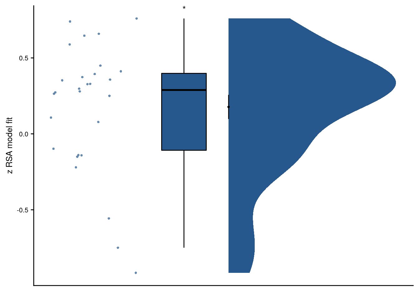
Supplemental Figure
Let’s compose a figure from the above plots to summarize these results of the control analyses for the same-sequence effects.
layout = "
AAAABDD
AAAACDD"
sfig <- sfiga + sfigb + sfigc + sfigd +
plot_layout(design = layout, guides = 'collect') &
theme(text = element_text(size=10, family = font2use),
axis.text = element_text(size=8),
legend.position = "bottom") &
plot_annotation(theme = theme(plot.margin = margin(t=-3, r=-6, b=-7, l=-6, unit="pt")),
tag_levels = 'A')
sfig[[4]] <- sfig[[4]] + theme(legend.position = "none")
# save and print to screen
fn <- here("figures", "sf05")
ggsave(paste0(fn, ".pdf"), plot=sfig, units = "cm",
width = 17.4, height = 10, dpi = "retina", device = cairo_pdf)
ggsave(paste0(fn, ".png"), plot=sfig, units = "cm",
width = 17.4, height = 10, dpi = "retina", device = "png")
Supplemental Figure 5. The relationship of virtual time and hippocampal pattern similarity change is not driven by the first and last event of a sequence. A. Z-values from the summary statistics approach show a significant positive effect of virtual time on pattern similarity change in the anterior hippcampus when competing for variance with a control predictor of no interest accounting for variance explained by whether pairs of events were made up from the first and last event of a sequence or not. B, C. Fixed effect estimate with confidence intervals (B) and estimated marginal means (C) visualize the results of the corresponding mixed model. D. We implemented participant-specific regression analyses with order and real time distances as predictors of hippocampal pattern similarity change. The plot shows a significant effect of virtual temporal distances when tested on the residuals of these linear models. Thus, variance that cannot be explained by the other time metrics can be accounted for by virtual temporal distances. This analysis was conducted only using the summary statistics approach because the residuals of a mixed model are more difficult to interpret than those of participant-specific regression analyses using ordinary least squares. A, D. Circles show individual participant Z-values from the summary statistics approach; boxplot shows median and upper/lower quartile along with whiskers extending to most extreme data point within 1.5 interquartile ranges above/below the upper/lower quartile; black circle with error bars corresponds to mean±S.E.M.; distribution shows probability density function of data points. * p<0.05
8.6 aHPC: virtual time across sequences
Having established that the anterior hippocampus forms sequence memories shaped by event relations in virtual time, we want to ask whether the hippocampus also generalizes across sequences. So next, we focus on pattern similarity changes for events that stem from different virtual days.
We separately tested the effect of virtual time for event pairs from the same or different sequences and thus use a Bonferroni-corrected α-level of 0.025 for these tests.
Summary statistics
set.seed(103) # set seed for reproducibility
# run a group-level t-test on the RSA fits from the first level in aHPC for across-day
stats <- rsa_fit %>%
filter(roi == "aHPC_lr", same_day == FALSE) %>%
select(z_virtual_time) %>%
paired_t_perm_jb (., n_perm = n_perm)
# Cohen's d with Hedges' correction for one sample using non-central t-distribution for CI
d<-cohen.d(d=(rsa_fit %>% filter(roi == "aHPC_lr", same_day == FALSE))$z_virtual_time, f=NA, paired=TRUE, hedges.correction=TRUE, noncentral=TRUE)
stats$d <- d$estimate
stats$dCI_low <- d$conf.int[[1]]
stats$dCI_high <- d$conf.int[[2]]
# print results
huxtable(stats) %>% theme_article()| estimate | statistic | p.value | p_perm | parameter | conf.low | conf.high | method | alternative | d | dCI_low | dCI_high |
|---|---|---|---|---|---|---|---|---|---|---|---|
| -0.5 | -2.65 | 0.0133 | 0.0128 | 27 | -0.887 | -0.113 | One Sample t-test | two.sided | -0.486 | -0.906 | -0.105 |
Summary Statistics: t-test against 0 for virtual time across sequences in aHPC
t27=-2.65, p=0.013, d=-0.49, 95% CI [-0.91, -0.10]
# select the data to plot
plot_dat <- rsa_fit %>% filter(roi == "aHPC_lr", same_day == FALSE)
ggplot(plot_dat, aes(x=1, y=z_virtual_time, fill = roi, color = roi)) +
gghalves::geom_half_violin(position=position_nudge(0.1),
side = "r", color = NA) +
geom_point(aes(x = 0.8, y = z_virtual_time), alpha = 0.7,
position = position_jitter(width = .1, height = 0),
shape=16, size = 1) +
geom_boxplot(position = position_nudge(x = 0, y = 0),
width = .1, colour = "black", outlier.shape = NA) +
stat_summary(fun = mean, geom = "point", size = 1, shape = 16,
position = position_nudge(.1), colour = "black") +
stat_summary(fun.data = mean_se, geom = "errorbar",
position = position_nudge(.1), colour = "black", width = 0, size = 0.5)+
scale_color_manual(values=unname(aHPC_colors["across_main"])) +
scale_fill_manual(values=unname(aHPC_colors["across_main"])) +
ylab('z RSA model fit') + xlab(element_blank()) +
guides(fill = "none", color = "none") +
annotate(geom = "text", x = 1, y = Inf, label = "**", hjust = 0.5, vjust = 1, size = 8/.pt, family=font2use) +
theme_cowplot() +
theme(text = element_text(size=10), axis.text = element_text(size=8),
legend.position = "none",
axis.ticks.x = element_blank(), axis.text.x = element_blank())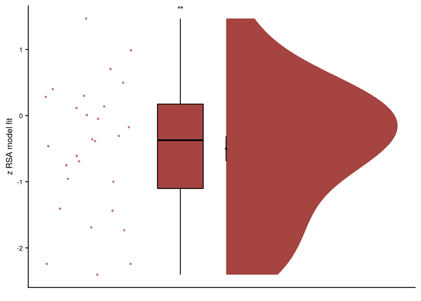
Linear Mixed Effects
Here, we fit a model with virtual time as the predictor for pattern similarity change for the across-day comparisons in the anterior hippocampus.
We start with a full random effects structure including random slopes and random intercepts for each subject. We reduce the random effects structure, but unfortunately even a simple model with only random slopes for the effect of virtual time results in a singular fit warning; even when trying different optimizers. We keep the random slopes to account for the within-subject dependencies in the data.
# extract the comparisons from different days
rsa_dat_diff_day <- rsa_dat %>%
filter(roi == "aHPC_lr", same_day == FALSE)
# define the full model with virtual time difference as
# fixed effect and by-subject random slopes and random intercepts --> singular fit
formula <- "ps_change ~ vir_time_diff + (1 + vir_time_diff | sub_id)"
lmm_full <- lme4::lmer(formula, data = rsa_dat_diff_day, REML = FALSE)## boundary (singular) fit: see ?isSingular# remove correlation --> still singular
formula <- "ps_change ~ vir_time_diff + (1 + vir_time_diff || sub_id)"
lmm_full <- lme4::lmer(formula, data = rsa_dat_diff_day, REML = FALSE)## boundary (singular) fit: see ?isSingular# only random slopes
set.seed(389) # set seed for reproducibility
formula <- "ps_change ~ vir_time_diff + (0 + vir_time_diff | sub_id)"
lmm_full <- lme4::lmer(formula, data = rsa_dat_diff_day, REML = FALSE,
#control = lmerControl(optimizer ='optimx', optCtrl=list(method='nlminb'))
#control = lmerControl(optimizer ="bobyqa", optCtrl=list(maxfun=40000))
control = lmerControl(optimizer ='nloptwrap',
optCtrl=list(method='NLOPT_LN_NELDERMEAD', maxfun=100000))
)## boundary (singular) fit: see ?isSingularsummary(lmm_full, corr = FALSE)## Linear mixed model fit by maximum likelihood ['lmerMod']
## Formula: ps_change ~ vir_time_diff + (0 + vir_time_diff | sub_id)
## Data: rsa_dat_diff_day
## Control: lmerControl(optimizer = "nloptwrap", optCtrl = list(method = "NLOPT_LN_NELDERMEAD", maxfun = 1e+05))
##
## AIC BIC logLik deviance df.resid
## -29625.4 -29600.0 14816.7 -29633.4 4196
##
## Scaled residuals:
## Min 1Q Median 3Q Max
## -4.3020 -0.6877 0.0324 0.6564 3.5548
##
## Random effects:
## Groups Name Variance Std.Dev.
## sub_id vir_time_diff 0.00e+00 0.000000
## Residual 5.05e-05 0.007107
## Number of obs: 4200, groups: sub_id, 28
##
## Fixed effects:
## Estimate Std. Error t value
## (Intercept) -6.075e-05 1.098e-04 -0.553
## vir_time_diff -2.745e-04 1.096e-04 -2.505
## convergence code: 0
## boundary (singular) fit: see ?isSingular# tidy summary of the fixed effects that calculates 95% CIs
lmm_full_bm <- broom.mixed::tidy(lmm_full, effects = "fixed",
conf.int=TRUE, conf.method="profile",
optimizer = 'nloptwrap')## Computing profile confidence intervals ...# tidy summary of the random effects
lmm_full_bm_re <- broom.mixed::tidy(lmm_full, effects = "ran_pars")
# one way of testing for significance is by comparing the likelihood against a simpler model.
# Here, we drop the effect of virtual time difference and run an ANOVA. See e.g. Bodo Winter tutorial
set.seed(328) # set seed for reproducibility
formula <- "ps_change ~ 1 + (0 + vir_time_diff | sub_id)"
lmm_no_vir_time <- lme4::lmer(formula, data = rsa_dat_diff_day, REML = FALSE)
lmm_aov <-anova(lmm_no_vir_time, lmm_full)Mixed Model: Fixed effect of virtual time across sequences on aHPC pattern similarity change \(\chi^2\)(1)=6.01, p=0.014
Make mixed model summary table that includes overview of fixed and random effects as well as the model comparison to the nested (reduced) model.
fe_names <- c("intercept", "virtual time")
re_groups <- c(rep("participant",1), "residual")
re_names <- c("virtual time (SD)", "SD")
lmm_hux <- make_lme_huxtable(fix_df=lmm_full_bm,
ran_df = lmm_full_bm_re,
aov_mdl = lmm_aov,
fe_terms =fe_names,
re_terms = re_names,
re_groups = re_groups,
lme_form = gsub(" ", "", paste0(deparse(formula(lmm_full)),
collapse = "", sep="")),
caption = "Mixed Model: Virtual time explains representational change for different-sequence events in the anterior hippocampus")
# convert the huxtable to a flextable for word export
stable_lme_aHPC_virtime_diff_seq <- convert_huxtable_to_flextable(ht = lmm_hux)
# print to screen
theme_article(lmm_hux)| fixed effects | ||||||
|---|---|---|---|---|---|---|
| term | estimate | SE | t-value | 95% CI | ||
| intercept | -0.000061 | 0.000110 | -0.55 | -0.000276 | 0.000155 | |
| virtual time | -0.000275 | 0.000110 | -2.51 | -0.000491 | -0.000058 | |
| random effects | ||||||
| group | term | estimate | ||||
| participant | virtual time (SD) | 0.000000 | ||||
| residual | SD | 0.007107 | ||||
| model comparison | ||||||
| model | npar | AIC | LL | X2 | df | p |
| reduced model | 3 | -29621.39 | 14813.69 | |||
| full model | 4 | -29625.40 | 14816.70 | 6.01 | 1 | 0.014 |
| model: ps_change~vir_time_diff+(0+vir_time_diff|sub_id); SE: standard error, CI: confidence interval, SD: standard deviation, npar: number of parameters, LL: log likelihood, df: degrees of freedom, corr.: correlation | ||||||
### PLOTS
lmm_full_bm <- lmm_full_bm %>%
mutate(term=as.factor(term))
# dot plot of Fixed Effect Coefficients with CIs
sfigmm_g <-ggplot(data = lmm_full_bm[2,], aes(x = term, color = term)) +
geom_hline(yintercept = 0, colour="black", linetype="dotted") +
geom_errorbar(aes(ymin = conf.low, ymax = conf.high, width = NA), size = 0.5) +
geom_point(aes(y = estimate), shape = 16, size = 1) +
scale_fill_manual(values = unname(aHPC_colors["across_main"])) +
scale_color_manual(values = unname(aHPC_colors["across_main"]), labels = c("virtual time (diff. seq.)"), name = element_blank()) +
labs(x = element_blank(), y = "fixed effect\nestimate", color = "") +
guides(fill = "none", color=guide_legend(override.aes=list(fill=NA, alpha = 1, size=2, linetype=0))) +
annotate(geom = "text", x = 1, y = Inf, label = "*", hjust = 0.5, vjust = 1, size = 8/.pt, family=font2use) +
theme_cowplot() +
theme(legend.position = "none", axis.text.x=element_blank())
sfigmm_g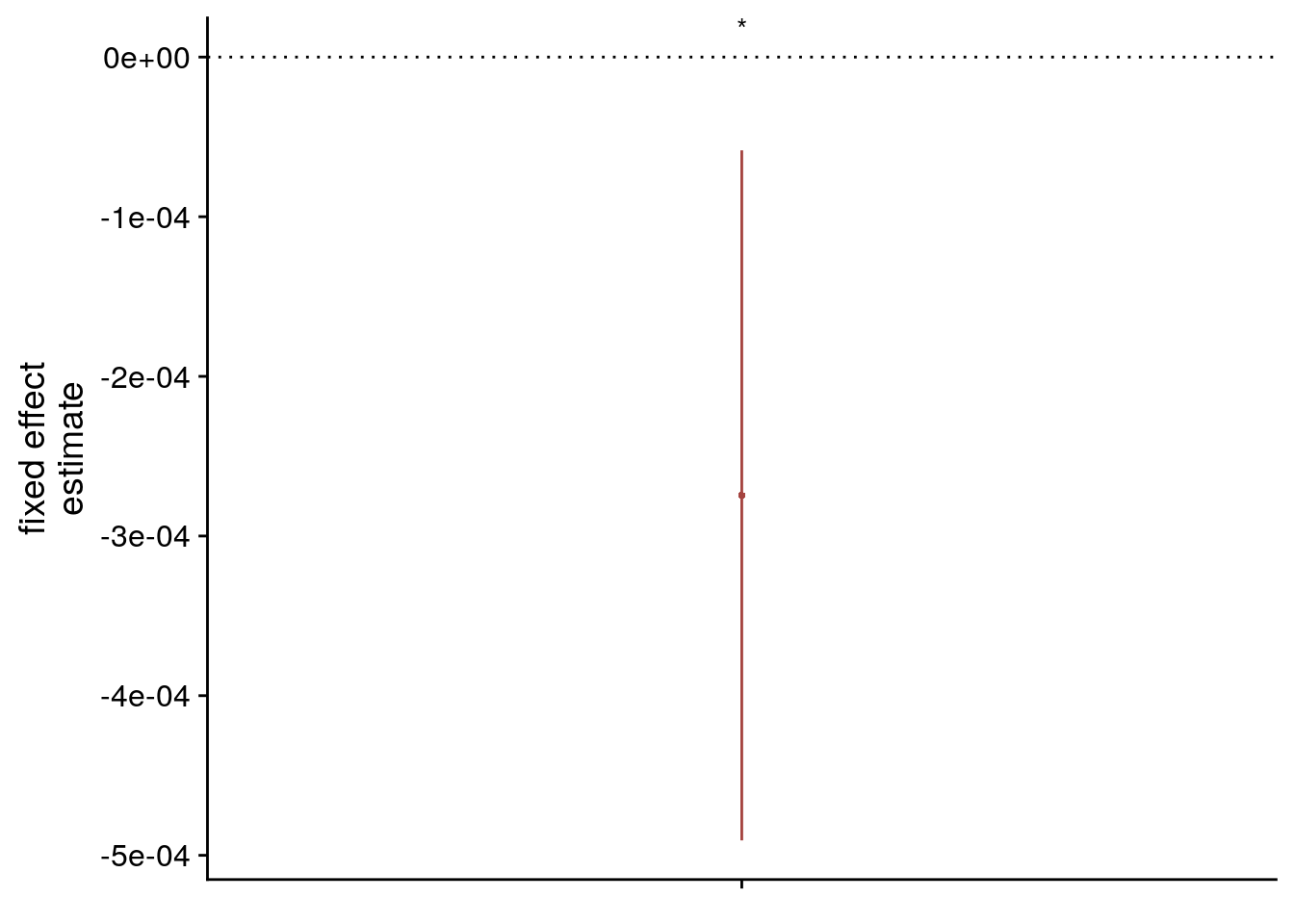
# estimate marginal means for each model term by omitting the terms argument
lmm_full_emm <- ggeffects::ggpredict(lmm_full, ci.lvl = 0.95) %>%
ggeffects::get_complete_df()
# plot marginal means
sfigmm_h <- ggplot(data = lmm_full_emm[lmm_full_emm$group == "vir_time_diff",], aes(color = group)) +
geom_line(aes(x, predicted)) +
geom_ribbon(aes(x, ymin = conf.low, ymax = conf.high, fill = group), alpha = .2, linetype=0) +
scale_color_manual(values = unname(aHPC_colors["across_main"]),
name = element_blank(), labels = "virtual time") +
scale_fill_manual(values = unname(aHPC_colors["across_main"])) +
ylab('estimated\nmarginal means') +
xlab('z time metric') +
#ggtitle("Estimated marginal means") +
guides(fill= "none", color= "none") +
theme_cowplot() +
theme(legend.position = "none")
sfigmm_h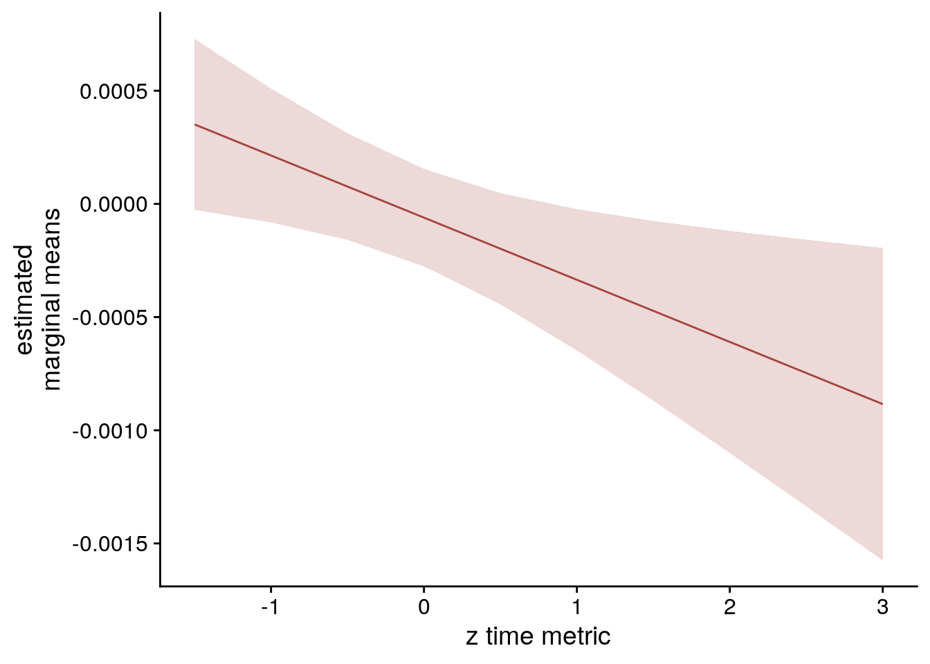
LME model assumptions
lmm_diagplots_jb(lmm_full)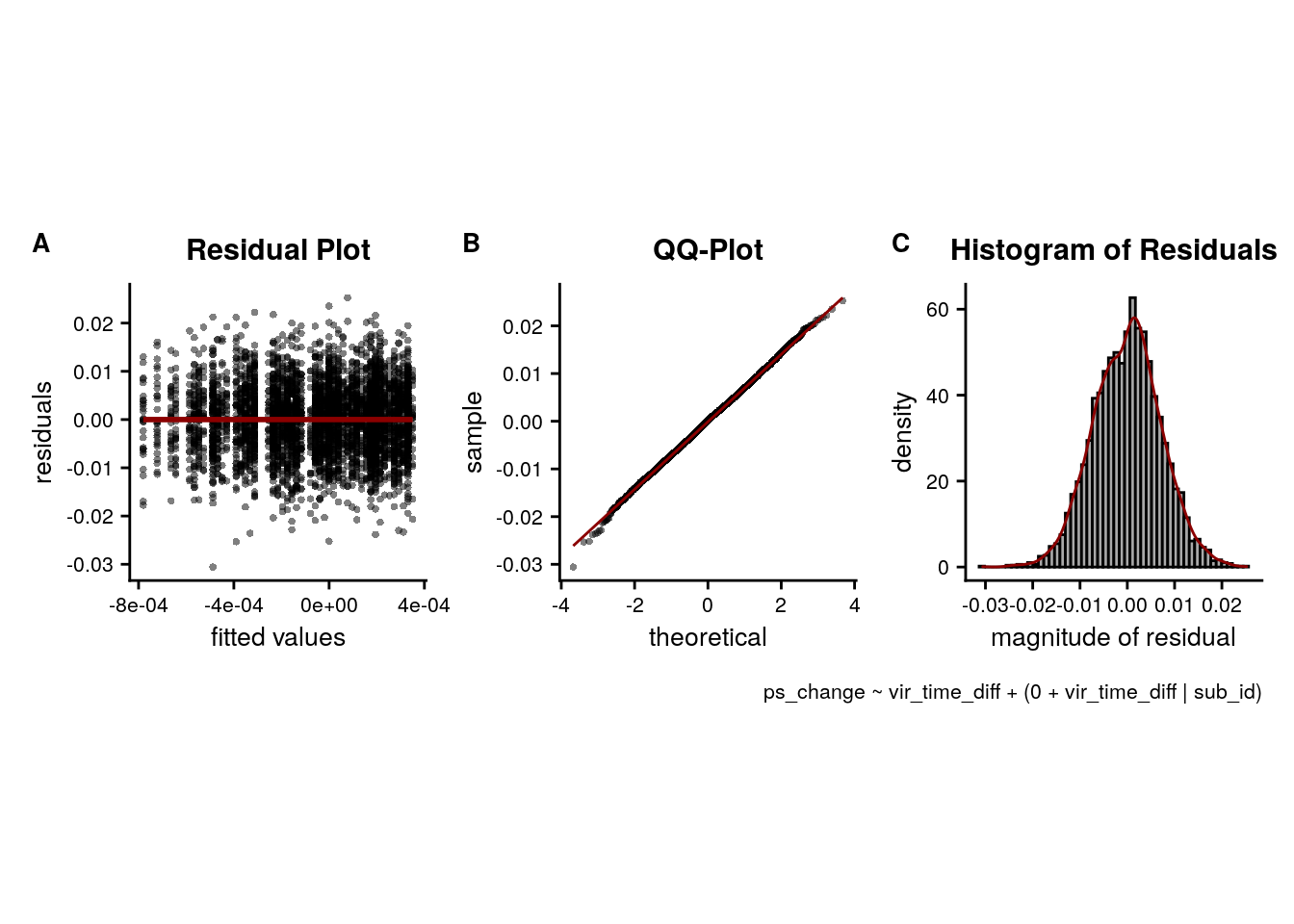
Representational Change Visualization
To illustrate the effect in a simpler way, we average pattern similarity changes based on a median split of events, separately for events from the same and from different sequences.
# Test pattern similarity for different-sequence events separated by high vs. low temporal distances
set.seed(209) # set seed for reproducibility
stats_diff_day_high_low <- paired_t_perm_jb(ps_change_means[ps_change_means$same_day=="different day" &
ps_change_means$temp_dist_f == "high",]$ps_change -
ps_change_means[ps_change_means$same_day=="different day" &
ps_change_means$temp_dist_f == "low",]$ps_change)
# Cohen's d with Hedges' correction for paired samples using non-central t-distribution for CI
d<-cohen.d(d=ps_change_means[ps_change_means$same_day=="different day" & ps_change_means$temp_dist_f == "high",]$ps_change,
f=ps_change_means[ps_change_means$same_day=="different day" & ps_change_means$temp_dist_f == "low",]$ps_change,
paired=TRUE, pooled=TRUE, hedges.correction=TRUE, noncentral=TRUE)
stats_diff_day_high_low$d <- d$estimate
stats_diff_day_high_low$dCI_low <- d$conf.int[[1]]
stats_diff_day_high_low$dCI_high <- d$conf.int[[2]]
huxtable(stats_diff_day_high_low) %>% theme_article()| estimate | statistic | p.value | p_perm | parameter | conf.low | conf.high | method | alternative | d | dCI_low | dCI_high |
|---|---|---|---|---|---|---|---|---|---|---|---|
| -0.000711 | -3.26 | 0.00304 | 0.0025 | 27 | -0.00116 | -0.000263 | One Sample t-test | two.sided | -0.89 | -1.03 | -0.209 |
To visualize the effect, lets make a plot of the raw pattern similarity change for high vs. low temporal distances.
f5b <- ggplot(data=ps_change_means %>% filter(same_day == "different day"), aes(x=temp_dist, y=ps_change, fill = same_day, color = same_day)) +
gghalves::geom_half_violin(data = ps_change_means %>% filter(same_day == "different day", temp_dist_f == "low"),
aes(x=temp_dist, y=ps_change),
position=position_nudge(-0.1),
side = "l", color = NA) +
gghalves::geom_half_violin(data = ps_change_means %>% filter(same_day == "different day", temp_dist_f == "high"),
aes(x=temp_dist, y=ps_change),
position=position_nudge(0.1),
side = "r", color = NA) +
geom_boxplot(aes(group = temp_dist),width = .1, colour = "black", outlier.shape = NA) +
geom_line(aes(x = x_jit, group=sub_id,), color = ultimate_gray,
position = position_nudge(c(0.15, -0.15))) +
geom_point(aes(x=x_jit), position = position_nudge(c(0.15, -0.15)),
shape=16, size = 1) +
stat_summary(fun = mean, geom = "point", size = 1, shape = 16,
position = position_nudge(c(-0.1, 0.1)), colour = "black") +
stat_summary(fun.data = mean_se, geom = "errorbar",
position = position_nudge(c(-0.1, 0.1)), colour = "black", width = 0, size = 0.5) +
scale_fill_manual(values = unname(aHPC_colors["across_main"])) +
scale_color_manual(values = unname(aHPC_colors["across_main"]), name = "different sequence", labels = "virtual time") +
scale_x_continuous(breaks = c(1,2), labels=c("low", "high")) +
annotate(geom = "text", x = 1.5, y = Inf, label = 'underline(" ** ")',
hjust = 0.5, vjust=1, size = 8/.pt, family=font2use, parse=TRUE) +
ylab('pattern similarity change') + xlab('virtual temporal distance') +
guides(fill= "none", color=guide_legend(override.aes=list(fill=NA, alpha = 1, size=2), title.position = "left")) +
theme_cowplot() +
theme(text = element_text(size=10), axis.text = element_text(size=8),
legend.position = "none", strip.background = element_blank(), strip.text = element_blank())
f5b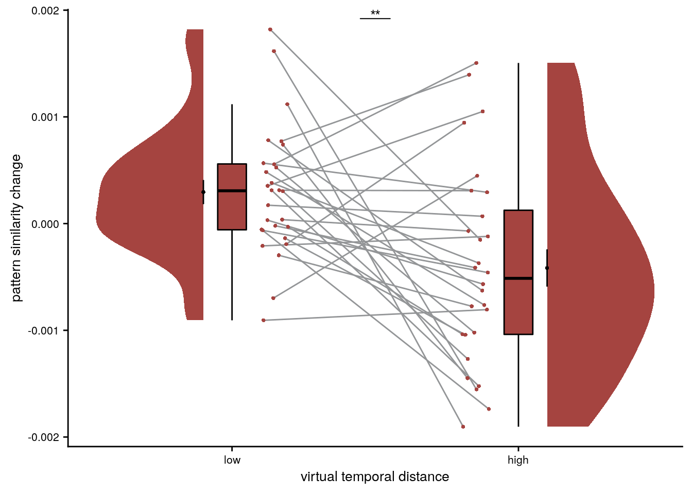
# save source data
source_dat <-ggplot_build(f5b)$data[[4]]
readr::write_tsv(source_dat %>% select(x,y, group),
file = file.path(dirs$source_dat_dir, "f5b.txt"))Summary Statistics: paired t-test for aHPC pattern similarity changes for high vs. low temporal distances for different sequence events t27=-3.26, p=0.002, d=-0.89, 95% CI [-1.03, -0.21]
8.7 aHPC: virtual time across sequence when including order & real time
We also test whether virtual time predicts aHPC pattern similarity changes for event pairs from different sequences when including order and real time in the model
Summary Statistics
# SUMMARY STATS AHPC WITH ORDER AND REAL TIME
set.seed(59) # set seed for reproducibility
# extract all comparisons from the same day
rsa_dat_diff_day_aHPC <- rsa_dat %>%
filter(roi == "aHPC_lr", same_day == FALSE)
# do RSA using linear model and calculate z-score for model fit from permutations
rsa_fit_aHPC_mult_reg <- rsa_dat_diff_day_aHPC %>% group_by(sub_id) %>%
# run the linear model
do(z = lm_perm_jb(in_dat = .,
lm_formula = "ps_change ~ vir_time_diff + order_diff + real_time_diff",
nsim = n_perm)) %>%
mutate(z = list(setNames(z, c("z_intercept", "z_virtual_time", "z_order", "z_real_time")))) %>%
unnest_longer(z) %>%
filter(z_id != "z_intercept")
# run group-level t-tests on the RSA fits from the first level in aHPC for within-day
stats <- rsa_fit_aHPC_mult_reg %>%
filter(z_id =="z_virtual_time") %>%
select(z) %>%
paired_t_perm_jb (., n_perm = n_perm)
# find outliers
is_outlier <- function(x) {
return(x < quantile(x, 0.25) - 1.5 * IQR(x) | x > quantile(x, 0.75) + 1.5 * IQR(x))
}
out_ind <- is_outlier(rsa_fit_aHPC_mult_reg$z[rsa_fit_aHPC_mult_reg$z_id == "z_virtual_time"])
out_sub <- subjects[out_ind]
# run second-level analysis on data points that are not outliers
set.seed(123) # set seed for reproducibility
stats <- rsa_fit_aHPC_mult_reg %>%
filter(sub_id != out_sub, z_id == "z_virtual_time") %>%
select("z") %>%
paired_t_perm_jb(., n_perm = n_perm)
huxtable(stats) %>% theme_article()| estimate | statistic | p.value | p_perm | parameter | conf.low | conf.high | method | alternative |
|---|---|---|---|---|---|---|---|---|
| -0.418 | -2.62 | 0.0146 | 0.0155 | 26 | -0.746 | -0.0897 | One Sample t-test | two.sided |
# Cohen's d with Hedges' correction for one sample using non-central t-distribution for CI
d<-cohen.d(d=(rsa_fit_aHPC_mult_reg %>% filter(z_id == "z_virtual_time", sub_id != out_sub))$z, f=NA, paired=TRUE, hedges.correction=TRUE, noncentral=TRUE)
stats$d <- d$estimate
stats$dCI_low <- d$conf.int[[1]]
stats$dCI_high <- d$conf.int[[2]]
# print results
huxtable(stats) %>% theme_article()| estimate | statistic | p.value | p_perm | parameter | conf.low | conf.high | method | alternative | d | dCI_low | dCI_high |
|---|---|---|---|---|---|---|---|---|---|---|---|
| -0.418 | -2.62 | 0.0146 | 0.0155 | 26 | -0.746 | -0.0897 | One Sample t-test | two.sided | -0.489 | -0.918 | -0.1 |
Summary Statistics: t-test against 0 for virtual time across sequences in aHPC with order and real time in the model
t26=-2.62, p=0.015, d=-0.49, 95% CI [-0.92, -0.10]
# make z_id a factor and reorder it
rsa_fit_aHPC_mult_reg <- rsa_fit_aHPC_mult_reg %>% mutate(
z_id = factor(z_id, levels = c("z_virtual_time", "z_order", "z_real_time")))
# raincloud plot
sfig6_a <- ggplot(rsa_fit_aHPC_mult_reg, aes(x=z_id, y=z, fill = z_id, colour = z_id)) +
gghalves::geom_half_violin(position=position_nudge(0.1),
side = "r", color = NA) +
geom_point(aes(x = as.numeric(z_id)-0.2), alpha = 0.7,
position = position_jitter(width = .1, height = 0),
shape=16, size = 1) +
geom_boxplot(position = position_nudge(x = 0, y = 0),
width = .1, colour = "black", outlier.shape = NA) +
stat_summary(fun = mean, geom = "point", size = 1, shape = 16,
position = position_nudge(.1), colour = "black") +
stat_summary(fun.data = mean_se, geom = "errorbar",
position = position_nudge(.1), colour = "black", width = 0, size = 0.5)+
ylab('z RSA model fit') + xlab('time metric') +
scale_x_discrete(labels = c("virtual time", "order", "real time")) +
scale_color_manual(values = c(unname(aHPC_colors["across_main"]), time_colors[c(2,3)]), name = "time metric",
labels = c("virtual", "order", "real")) +
scale_fill_manual(values = c(unname(aHPC_colors["across_main"]), time_colors[c(2,3)])) +
guides(fill= "none", color=guide_legend(override.aes=list(fill=NA, alpha = 1, size=2))) +
annotate(geom = "text", x = 1, y = Inf, label = "*", hjust = 0.5, vjust = 1, size = 8/.pt, family=font2use) +
theme_cowplot() +
theme(text = element_text(size=10), axis.text = element_text(size=8),
legend.position = "none")
sfig6_a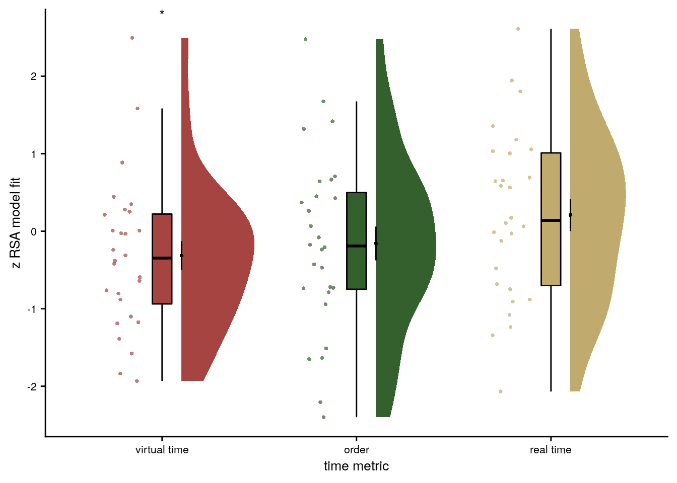
Linear Mixed Effects
# MIXED EFFECT AHPC WITH ORDER AND REAL TIME
set.seed(87) # set seed for reproducibility
# extract the comparisons from different days, exclude outlier
rsa_dat_diff_day <- rsa_dat %>% filter(roi == "aHPC_lr", same_day == FALSE, sub_id != out_sub)
# define the full model with virtual time difference, order difference and real time difference as
# fixed effects and random intercepts and random slopes for all effects
# fails to converge and is singular after restart
formula <- "ps_change ~ vir_time_diff + order_diff + real_time_diff + (1+vir_time_diff + order_diff + real_time_diff | sub_id)"
lmm_full <- lme4::lmer(formula, data = rsa_dat_diff_day, REML = FALSE)## boundary (singular) fit: see ?isSingular#lmm_full <- update(lmm_full, start=getME(lmm_full, "theta"))
# remove the correlation between random slopes and random intercepts
formula <- "ps_change ~ vir_time_diff + order_diff + real_time_diff + (1+vir_time_diff + order_diff + real_time_diff || sub_id)"
lmm_full <- lme4::lmer(formula, data = rsa_dat_diff_day, REML = FALSE)## boundary (singular) fit: see ?isSingular# thus we reduce the random effect structure by excluding random slopes for the fixed effects of no interest
# as above this results in a singular fit (the random intercept variance estimated to be 0)
formula <- "ps_change ~ vir_time_diff + order_diff + real_time_diff + (1+vir_time_diff | sub_id)"
lmm_full <- lme4::lmer(formula, data = rsa_dat_diff_day, REML = FALSE)## boundary (singular) fit: see ?isSingular# next step is to remove the correlation between random slopes and random intercepts
formula <- "ps_change ~ vir_time_diff + order_diff + real_time_diff + (1+vir_time_diff || sub_id)"
lmm_full <- lme4::lmer(formula, data = rsa_dat_diff_day, REML = FALSE)## boundary (singular) fit: see ?isSingular# we thus reduce further and keep only the random slopes for virtual time differences
# but the model converges with the warning about the singular fit
set.seed(332) # set seed for reproducibility
formula <- "ps_change ~ vir_time_diff + order_diff + real_time_diff + (0 + vir_time_diff | sub_id)"
lmm_full <- lme4::lmer(formula, data = rsa_dat_diff_day, REML = FALSE)## boundary (singular) fit: see ?isSingularsummary(lmm_full, corr = FALSE)## Linear mixed model fit by maximum likelihood ['lmerMod']
## Formula: ps_change ~ vir_time_diff + order_diff + real_time_diff + (0 + vir_time_diff | sub_id)
## Data: rsa_dat_diff_day
##
## AIC BIC logLik deviance df.resid
## -28597.1 -28559.3 14304.6 -28609.1 4044
##
## Scaled residuals:
## Min 1Q Median 3Q Max
## -4.2924 -0.6858 0.0382 0.6566 3.6191
##
## Random effects:
## Groups Name Variance Std.Dev.
## sub_id vir_time_diff 0.000e+00 0.000000
## Residual 5.008e-05 0.007077
## Number of obs: 4050, groups: sub_id, 27
##
## Fixed effects:
## Estimate Std. Error t value
## (Intercept) -0.0001006 0.0001115 -0.902
## vir_time_diff -0.0006234 0.0002944 -2.118
## order_diff -0.0003476 0.0004777 -0.728
## real_time_diff 0.0007023 0.0005288 1.328
## convergence code: 0
## boundary (singular) fit: see ?isSingular# tidy summary of the fixed effects that calculates 95% CIs
lmm_full_bm <- broom.mixed::tidy(lmm_full, effects = "fixed", conf.int=TRUE, conf.method="profile")## Computing profile confidence intervals ...# tidy summary of the random effects
lmm_full_bm_re <- broom.mixed::tidy(lmm_full, effects = "ran_pars")
# one way of testing for significance is by comparing the likelihood against a simpler model.
# Here, we drop the effect of virtual time difference and run an ANOVA. See e.g. Bodo Winter tutorial
set.seed(321) # set seed for reproducibility
formula <- "ps_change ~ order_diff + real_time_diff + (0 + vir_time_diff | sub_id)"
lmm_no_vir_time <- lme4::lmer(formula, data = rsa_dat_diff_day, REML = FALSE)## boundary (singular) fit: see ?isSingularlmm_aov <- anova(lmm_no_vir_time, lmm_full)
lmm_aov| npar | AIC | BIC | logLik | deviance | Chisq | Df | Pr(>Chisq) |
|---|---|---|---|---|---|---|---|
| 5 | -2.86e+04 | -2.86e+04 | 1.43e+04 | -2.86e+04 | |||
| 6 | -2.86e+04 | -2.86e+04 | 1.43e+04 | -2.86e+04 | 4.48 | 1 | 0.0343 |
Mixed Model: Fixed effect of virtual time on aHPC across-sequence pattern similarity change with order and real time in model \(\chi^2\)(1)=4.48, p=0.034
Make mixed model summary table that includes overview of fixed and random effects as well as the model comparison to the nested (reduced) model.
fe_names <- c("intercept", "virtual time", "order", "real time")
re_groups <- c(rep("participant",1), "residual")
re_names <- c("virtual time (SD)", "SD")
lmm_hux <- make_lme_huxtable(fix_df=lmm_full_bm,
ran_df = lmm_full_bm_re,
aov_mdl = lmm_aov,
fe_terms =fe_names,
re_terms = re_names,
re_groups = re_groups,
lme_form = gsub(" ", "", paste0(deparse(formula(lmm_full)),
collapse = "", sep="")),
caption = "Mixed Model: Virtual time explains representational change for different-sequence events in the anterior hippocampus when including order and real time in the model")
# convert the huxtable to a flextable for word export
stable_lme_aHPC_virtime_diff_seq_time_metrics <- convert_huxtable_to_flextable(ht = lmm_hux)
# print to screen
theme_article(lmm_hux)| fixed effects | ||||||
|---|---|---|---|---|---|---|
| term | estimate | SE | t-value | 95% CI | ||
| intercept | -0.000101 | 0.000112 | -0.90 | -0.000319 | 0.000118 | |
| virtual time | -0.000623 | 0.000294 | -2.12 | -0.001201 | -0.000046 | |
| order | -0.000348 | 0.000478 | -0.73 | -0.001284 | 0.000589 | |
| real time | 0.000702 | 0.000529 | 1.33 | -0.000334 | 0.001739 | |
| random effects | ||||||
| group | term | estimate | ||||
| participant | virtual time (SD) | 0.000000 | ||||
| residual | SD | 0.007077 | ||||
| model comparison | ||||||
| model | npar | AIC | LL | X2 | df | p |
| reduced model | 5 | -28594.64 | 14302.32 | |||
| full model | 6 | -28597.12 | 14304.56 | 4.48 | 1 | 0.034 |
| model: ps_change~vir_time_diff+order_diff+real_time_diff+(0+vir_time_diff|sub_id); SE: standard error, CI: confidence interval, SD: standard deviation, npar: number of parameters, LL: log likelihood, df: degrees of freedom, corr.: correlation | ||||||
Mixed model plots.
# set RNG
set.seed(23)
lmm_full_bm <- lmm_full_bm %>%
mutate(term=as.factor(term) %>%
factor(levels = c("vir_time_diff", "order_diff", "real_time_diff")))
# dot plot of Fixed Effect Coefficients with CIs
sfig6_b <- ggplot(data = lmm_full_bm[2:4,], aes(x = term, color = term)) +
geom_hline(yintercept = 0, colour="black", linetype="dotted") +
geom_errorbar(aes(ymin = conf.low, ymax = conf.high, width = NA), size = 0.5) +
geom_point(aes(y = estimate), shape = 16, size = 1) +
scale_fill_manual(values = c(unname(aHPC_colors["across_main"]), time_colors[c(2,3)])) +
scale_color_manual(values = c(unname(aHPC_colors["across_main"]), time_colors[c(2,3)]), labels = c("Virtual", "Order", "Real")) +
labs(x = "time metric", y = "fixed effect\nestimate", color = "Time Metric") +
guides(color = "none", fill = "none") +
annotate(geom = "text", x = 1, y = Inf, label = "*", hjust = 0.5, vjust = 1, size = 8/.pt, family=font2use) +
theme_cowplot() +
theme(plot.title = element_text(hjust = 0.5), axis.text.x=element_blank())
sfig6_b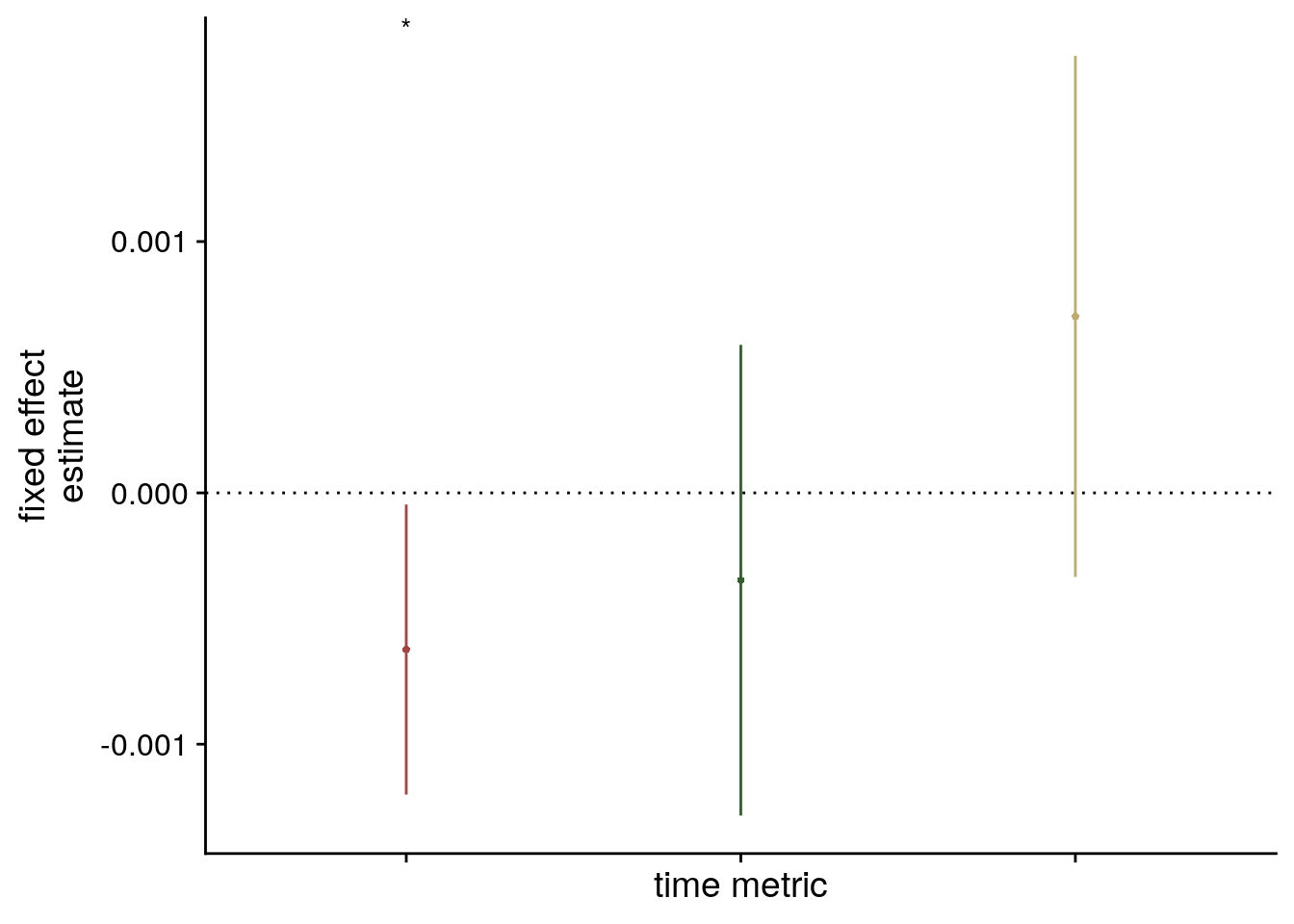
# estimate marginal means for each model term by omitting the terms argument
lmm_full_emm <- ggeffects::ggpredict(lmm_full, ci.lvl = 0.95) %>% get_complete_df
# convert the group variable to a factor to control the order of facets below
lmm_full_emm$group <- factor(lmm_full_emm$group, levels = c("vir_time_diff", "order_diff", "real_time_diff"))
# plot marginal means
sfig6_c <- ggplot(data = lmm_full_emm, aes(color = group)) +
geom_line(aes(x, predicted)) +
geom_ribbon(aes(x, ymin = conf.low, ymax = conf.high, fill = group), alpha = .2, linetype=0) +
scale_color_manual(values = c(unname(aHPC_colors["across_main"]), time_colors[c(2,3)]), name = element_blank(),
labels = c("virtual time", "order", "real time")) +
scale_fill_manual(values = c(unname(aHPC_colors["across_main"]), time_colors[c(2,3)])) +
ylab('estimated\nmarginal means') +
xlab('z time metric') +
guides(fill = "none", color= "none") +
theme_cowplot() +
theme(plot.title = element_text(hjust = 0.5), strip.background = element_blank(),
strip.text.x = element_blank())
sfig6_c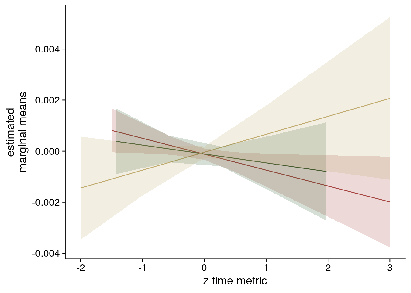
8.8 aHPC: virtual time within vs. across sequences
The previous results show positive correlations of pattern similarity change with temporal distances between event pairs from the same sequence and negative correlations with temporal distances when events are from different sequences. Next, we want to quantify whether these two modes of representation are significantly different from each other.
Second-level analysis
For the summary statistics approach, we run a permutation-based paired t-test to check for a difference in the effect of virtual time depending on whether we look at within vs. across sequences.
set.seed(105) # set seed for reproducibility
stats <- rsa_fit %>%
filter(roi=="aHPC_lr") %>%
# calculate difference between within- an across-day effect for each participant
group_by(sub_id) %>%
summarise(
same_day_diff = z_virtual_time[same_day==TRUE]-z_virtual_time[same_day==FALSE],
.groups = "drop") %>%
# test difference against 0
select(same_day_diff) %>%
paired_t_perm_jb (., n_perm = n_perm)
# Cohen's d with Hedges' correction for paired samples using non-central t-distribution for CI
d<-cohen.d(d=(rsa_fit %>% filter(roi == "aHPC_lr", same_day == TRUE))$z_virtual_time,
f=(rsa_fit %>% filter(roi == "aHPC_lr", same_day == FALSE))$z_virtual_time,
paired=TRUE, pooled =TRUE, hedges.correction=TRUE, noncentral=TRUE)
stats$d <- d$estimate
stats$dCI_low <- d$conf.int[[1]]
stats$dCI_high <- d$conf.int[[2]]
# print results
huxtable(stats) %>% theme_article()| estimate | statistic | p.value | p_perm | parameter | conf.low | conf.high | method | alternative | d | dCI_low | dCI_high |
|---|---|---|---|---|---|---|---|---|---|---|---|
| 1.12 | 3.71 | 0.000941 | 0.001 | 27 | 0.5 | 1.74 | One Sample t-test | two.sided | 1.05 | 0.287 | 1.13 |
Summary Statistics: paired t-test comparing effects of virtual time within and across sequences in aHPC
t27=3.71, p=0.001, d=1.05, 95% CI [0.29, 1.13]
To visualize the difference between the effects of virtual time for events from the same or different day, we create a pair of rainclouds facing each other. We use a custom jitter so that the length of lines connecting individual subject data points remains constant, thus keeping their slopes comparable.
# generate custom repeating jitter (multiply with -1/1 to shift towards each other)
plot_dat <- rsa_fit %>%
filter(roi=="aHPC_lr") %>%
mutate(
same_day_num = plyr::mapvalues(same_day, from = c("FALSE", "TRUE"),to = c(1,0)),
same_day_char = plyr::mapvalues(same_day, from = c("FALSE", "TRUE"),
to = c("different", "same")),
same_day_char = fct_relevel(same_day_char, c("same", "different")),
x_jit = as.numeric(same_day_char) + rep(jitter(rep(0,n_subs), amount=0.05), each=2) * rep(c(-1,1),n_subs))
f5a<- ggplot(data=plot_dat, aes(x=same_day_char, y=z_virtual_time, fill = same_day_char, color = same_day_char)) +
geom_boxplot(aes(group=same_day_char), position = position_nudge(x = 0, y = 0),
width = .1, colour = "black", outlier.shape = NA) +
scale_fill_manual(values = unname(c(aHPC_colors["within_main"], aHPC_colors["across_main"]))) +
scale_color_manual(values = unname(c(aHPC_colors["within_main"], aHPC_colors["across_main"])),
name = "sequence", labels=c("same", "different")) +
gghalves::geom_half_violin(data = plot_dat %>% filter(same_day == TRUE),
aes(x=same_day_char, y=z_virtual_time),
position=position_nudge(-0.1),
side = "l", color = NA) +
gghalves::geom_half_violin(data = plot_dat %>% filter(same_day == FALSE),
aes(x=same_day_char, y=z_virtual_time),
position=position_nudge(0.1),
side = "r", color = NA) +
stat_summary(fun = mean, geom = "point", size = 1, shape = 16,
position = position_nudge(c(-0.1, 0.1)), colour = "black") +
stat_summary(fun.data = mean_se, geom = "errorbar",
position = position_nudge(c(-0.1, 0.1)), colour = "black", width = 0, size = 0.5) +
geom_line(aes(x = x_jit, group=sub_id,), color = ultimate_gray,
position = position_nudge(c(0.15, -0.15))) +
geom_point(aes(x=x_jit, fill = same_day_char), position = position_nudge(c(-0.15, 0.15)),
shape=16, size = 1) +
ylab('z RSA model fit') + xlab('sequence') +
guides(fill = "none", color = "none") +
annotate(geom = "text", x = c(1, 2), y = Inf,
label = c('**', '*'),
hjust = 0.5, vjust = 1, size = 8/.pt, family=font2use) +
annotate(geom = "text", x = 1.5, y = Inf,
label = 'underline(" *** ")',
hjust = 0.5, vjust = 1, size = 8/.pt, family=font2use, parse = TRUE) +
theme_cowplot() +
theme(text = element_text(size=10), axis.text = element_text(size=8),
legend.position = "bottom")
f5a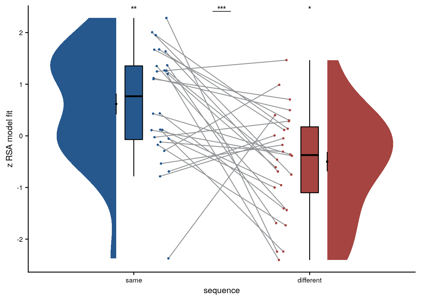
# save source data
source_dat <-ggplot_build(f5a)$data[[6]]
readr::write_tsv(source_dat %>% select(x,y, group),
file = file.path(dirs$source_dat_dir, "f5a.txt"))Linear Mixed Effects
Next, we test whether there is an interaction effect, i.e. we test whether the effect of virtual time on hippocampal pattern similarity change depends on whether we look at event pairs from the same vs. from different days.
We again have to reduce our model from the maximal random effects structure. We end up with a model that keeps only the random slopes for the interaction of virtual time and day. This is in keeping with the paper on random effect structures when testing interactions that emphasizes the importance of random slopes for the interaction of interest Barr, 2013, Frontiers Psychology.
# get the data
rsa_dat_aHPC <- rsa_dat %>% filter(roi == "aHPC_lr")
# test the interaction for aHPC
# maximal random effect structure --> singular fit
formula <- "ps_change ~ vir_time_diff * same_day_dv + (1 + vir_time_diff * same_day_dv | sub_id)"
lmm_full = lme4::lmer(formula, data=rsa_dat_aHPC, REML=FALSE)## boundary (singular) fit: see ?isSingular# no correlations with random intercept --> singular fit
formula <- "ps_change ~ vir_time_diff * same_day_dv + (1 + vir_time_diff * same_day_dv || sub_id)"
lmm_full = lme4::lmer(formula, data=rsa_dat_aHPC, REML=FALSE)## boundary (singular) fit: see ?isSingular# random intercepts and random slopes only for the critical interaction --> singular fit
formula <- "ps_change ~ vir_time_diff * same_day_dv + (1 + vir_time_diff : same_day_dv || sub_id)"
lmm_full = lme4::lmer(formula, data=rsa_dat_aHPC, REML=FALSE)## boundary (singular) fit: see ?isSingular# random slopes for critical interactions
set.seed(334) # set seed for reproducibility
formula <- "ps_change ~ vir_time_diff * same_day_dv + (0 + vir_time_diff : same_day_dv | sub_id)"
lmm_full = lme4::lmer(formula, data=rsa_dat_aHPC, REML=FALSE)
summary(lmm_full, corr = FALSE)## Linear mixed model fit by maximum likelihood ['lmerMod']
## Formula: ps_change ~ vir_time_diff * same_day_dv + (0 + vir_time_diff:same_day_dv | sub_id)
## Data: rsa_dat_aHPC
##
## AIC BIC logLik deviance df.resid
## -37581.7 -37542.3 18796.9 -37593.7 5314
##
## Scaled residuals:
## Min 1Q Median 3Q Max
## -4.3282 -0.6823 0.0196 0.6564 3.7447
##
## Random effects:
## Groups Name Variance Std.Dev.
## sub_id vir_time_diff:same_day_dv 3.083e-08 0.0001756
## Residual 4.993e-05 0.0070659
## Number of obs: 5320, groups: sub_id, 28
##
## Fixed effects:
## Estimate Std. Error t value
## (Intercept) -0.0001934 0.0001209 -1.600
## vir_time_diff 0.0002384 0.0001223 1.950
## same_day_dv -0.0001327 0.0001209 -1.098
## vir_time_diff:same_day_dv 0.0005129 0.0001267 4.049# tidy summary of the fixed effects that calculates 95% CIs
lmm_full_bm <- broom.mixed::tidy(lmm_full, effects = "fixed", conf.int=TRUE, conf.method="profile")## Computing profile confidence intervals ...# tidy summary of the random effects
lmm_full_bm_re <- broom.mixed::tidy(lmm_full, effects = "ran_pars")
# test against reduced model
set.seed(309) # set seed for reproducibility
lmm_reduced <- update(lmm_full, ~ . - vir_time_diff:same_day_dv)
lmm_aov <- anova(lmm_reduced, lmm_full)
# store for future use (MDS)
lmm_aHPC_interaction <- lmm_fullMixed Model: Fixed effect of interaction of virtual time with sequence identity on aHPC pattern similarity change \(\chi^2\)(1)=14.37, p=0.000
Make mixed model summary table that includes overview of fixed and random effects as well as the model comparison to the nested (reduced) model.
fe_names <- c("intercept", "virtual time", "day", "interaction virtual time and day")
re_groups <- c(rep("participant",1), "residual")
re_names <- c("interaction virtual time and day (SD)", "SD")
lmm_hux <- make_lme_huxtable(fix_df=lmm_full_bm,
ran_df = lmm_full_bm_re,
aov_mdl = lmm_aov,
fe_terms =fe_names,
re_terms = re_names,
re_groups = re_groups,
lme_form = gsub(" ", "", paste0(deparse(formula(lmm_full)),
collapse = "", sep="")),
caption = "Mixed Model: The effect of virtual time differs between same-sequence and different-sequence events in the anterior hippocampus")
# convert the huxtable to a flextable for word export
stable_lme_aHPC_virtime_same_vs_diff_seq <- convert_huxtable_to_flextable(ht = lmm_hux)
# print to screen
theme_article(lmm_hux)| fixed effects | ||||||
|---|---|---|---|---|---|---|
| term | estimate | SE | t-value | 95% CI | ||
| intercept | -0.000193 | 0.000121 | -1.60 | -0.000430 | 0.000044 | |
| virtual time | 0.000238 | 0.000122 | 1.95 | -0.000001 | 0.000478 | |
| day | -0.000133 | 0.000121 | -1.10 | -0.000370 | 0.000104 | |
| interaction virtual time and day | 0.000513 | 0.000127 | 4.05 | 0.000261 | 0.000765 | |
| random effects | ||||||
| group | term | estimate | ||||
| participant | interaction virtual time and day (SD) | 0.000176 | ||||
| residual | SD | 0.007066 | ||||
| model comparison | ||||||
| model | npar | AIC | LL | X2 | df | p |
| reduced model | 5 | -37569.38 | 18789.69 | |||
| full model | 6 | -37581.75 | 18796.87 | 14.37 | 1 | 1.50e-04 |
| model: ps_change~vir_time_diff*same_day_dv+(0+vir_time_diff:same_day_dv|sub_id); SE: standard error, CI: confidence interval, SD: standard deviation, npar: number of parameters, LL: log likelihood, df: degrees of freedom, corr.: correlation | ||||||
lmm_full_bm <- lmm_full_bm %>%
mutate(term=as.factor(term))
# dot plot of Fixed Effect Coefficients with CIs
sfigmm_i <- ggplot(data = lmm_full_bm[2:4,], aes(x = term, color = term)) +
geom_hline(yintercept = 0, colour="black", linetype="dotted") +
geom_errorbar(aes(ymin = conf.low, ymax = conf.high, width = NA), size = 0.5) +
geom_point(aes(y = estimate), shape = 16, size = 1) +
scale_fill_manual(values = c(rep("black",6), "#DD8D29")) +
scale_color_manual(values = c(ultimate_gray, time_within_across_color, day_time_int_color), name = element_blank(),
labels = c("sequence", "virtual time (all events)", "interaction")) +
labs(x = element_blank(), y = "fixed effect\nestimate") +
theme_cowplot() +
guides(fill = "none", color=guide_legend(override.aes=list(fill=NA, alpha = 1, size=2, linetype=0))) +
annotate(geom = "text", x = 3, y = Inf, label = "***", hjust = 0.5, vjust = 1, size = 8/.pt, family=font2use) +
theme(plot.title = element_text(hjust = 0.5), axis.text.x=element_blank(), legend.position = "bottom")
sfigmm_i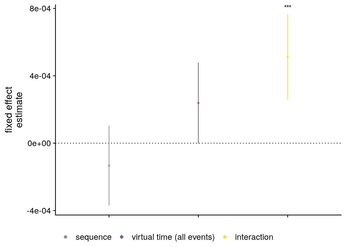
# estimate marginal means (& add factor for easier plotting)
hpc_emms <- ggeffects::ggpredict(lmm_full, terms = c("vir_time_diff", "same_day_dv")) %>%
as_tibble() %>%
mutate(day = factor(if_else(group == 1, true = "same day", false = "different day"),
levels = c("same day", "different day")))
# plot marginal means
sfigmm_j <- ggplot(hpc_emms, aes(x = x, y = predicted, colour = day, fill = day)) +
geom_ribbon(aes(ymin = conf.low, ymax = conf.high), alpha = .2, linetype=0) +
geom_line(size = 0.5) +
#geom_line(aes(linetype = day), size = 0.5) +
#scale_linetype_manual(values=c("solid", "2121")) +
scale_fill_manual(values = unname(c(aHPC_colors[c("within_main", "across_main")])), name = element_blank()) +
scale_color_manual(values = unname(c(aHPC_colors[c("within_main", "across_main")]))) +
ylab('estimated\nmarginal means') +
xlab('z virtual time') +
guides(fill = "none", color = "none", linetype = "none") +
theme_cowplot() +
theme(legend.title = element_blank())
sfigmm_j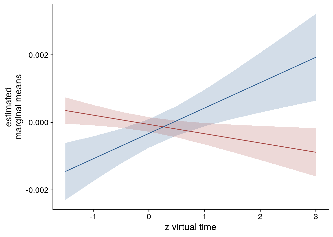
LME model assumptions
lmm_diagplots_jb(lmm_full)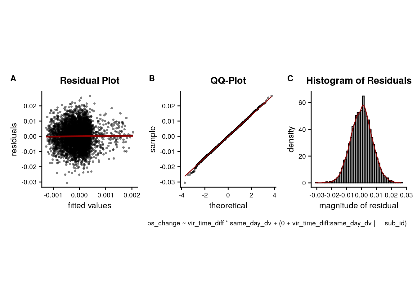
Interaction of sequence membership and order
# interaction of order and sequence (including only cirtical random slopes to avoid singular fit)
formula <- "ps_change ~ order_diff * same_day_dv + (0 + order_diff : same_day_dv | sub_id)"
lmm_full = lme4::lmer(formula, data=rsa_dat_aHPC, REML=FALSE)
lmm_reduced <- update(lmm_full, ~ . - order_diff:same_day_dv)
lmm_aov <- anova(lmm_reduced, lmm_full)
lmm_aov| npar | AIC | BIC | logLik | deviance | Chisq | Df | Pr(>Chisq) |
|---|---|---|---|---|---|---|---|
| 5 | -3.76e+04 | -3.75e+04 | 1.88e+04 | -3.76e+04 | |||
| 6 | -3.76e+04 | -3.75e+04 | 1.88e+04 | -3.76e+04 | 9.98 | 1 | 0.00158 |
Mixed Model: Fixed effect of interaction of order with sequence identity on aHPC pattern similarity change \(\chi^2\)(1)=9.98, p=0.002
Interaction of sequence membership and real time
# interaction of real time and sequence (including only cirtical random slopes to avoid singular fit)
formula <- "ps_change ~ real_time_diff * same_day_dv + (0 + real_time_diff : same_day_dv | sub_id)"
lmm_full = lme4::lmer(formula, data=rsa_dat_aHPC, REML=FALSE)
lmm_reduced <- update(lmm_full, ~ . - real_time_diff:same_day_dv)
lmm_aov <- anova(lmm_reduced, lmm_full)
lmm_aov| npar | AIC | BIC | logLik | deviance | Chisq | Df | Pr(>Chisq) |
|---|---|---|---|---|---|---|---|
| 5 | -3.76e+04 | -3.75e+04 | 1.88e+04 | -3.76e+04 | |||
| 6 | -3.76e+04 | -3.75e+04 | 1.88e+04 | -3.76e+04 | 9.27 | 1 | 0.00232 |
Mixed Model: Fixed effect of interaction of real time with sequence identity on aHPC pattern similarity change \(\chi^2\)(1)=9.27, p=0.002
Interaction of sequence membership and virtual time when including interactions with other time metrics
# test the interaction for aHPC
# maximal random effect structure --> singular fit
formula <- "ps_change ~ vir_time_diff * same_day_dv + order_diff:same_day_dv + real_time_diff:same_day_dv+ (1 + vir_time_diff * same_day_dv | sub_id)"
lmm_full = lme4::lmer(formula, data=rsa_dat_aHPC, REML=FALSE)## boundary (singular) fit: see ?isSingular# no correlations with random intercept --> singular fit
formula <- "ps_change ~ vir_time_diff * same_day_dv + order_diff:same_day_dv + real_time_diff:same_day_dv+ (1 + vir_time_diff * same_day_dv || sub_id)"
lmm_full = lme4::lmer(formula, data=rsa_dat_aHPC, REML=FALSE)## boundary (singular) fit: see ?isSingular# random intercepts and random slopes only for the critical interaction --> singular fit
formula <- "ps_change ~ vir_time_diff * same_day_dv + order_diff:same_day_dv + real_time_diff:same_day_dv+ (1 + vir_time_diff : same_day_dv || sub_id)"
lmm_full = lme4::lmer(formula, data=rsa_dat_aHPC, REML=FALSE)## boundary (singular) fit: see ?isSingular# random slopes for critical interactions
set.seed(334) # set seed for reproducibility
formula <- "ps_change ~ vir_time_diff * same_day_dv + order_diff:same_day_dv + real_time_diff:same_day_dv+ (0 + vir_time_diff : same_day_dv | sub_id)"
lmm_full = lme4::lmer(formula, data=rsa_dat_aHPC, REML=FALSE)
summary(lmm_full, corr = FALSE)## Linear mixed model fit by maximum likelihood ['lmerMod']
## Formula: ps_change ~ vir_time_diff * same_day_dv + order_diff:same_day_dv + real_time_diff:same_day_dv + (0 + vir_time_diff:same_day_dv | sub_id)
## Data: rsa_dat_aHPC
##
## AIC BIC logLik deviance df.resid
## -37579.5 -37526.9 18797.8 -37595.5 5312
##
## Scaled residuals:
## Min 1Q Median 3Q Max
## -4.3143 -0.6830 0.0224 0.6567 3.7470
##
## Random effects:
## Groups Name Variance Std.Dev.
## sub_id vir_time_diff:same_day_dv 3.092e-08 0.0001758
## Residual 4.991e-05 0.0070647
## Number of obs: 5320, groups: sub_id, 28
##
## Fixed effects:
## Estimate Std. Error t value
## (Intercept) -0.0001895 0.0001219 -1.554
## vir_time_diff 0.0002373 0.0001237 1.919
## same_day_dv -0.0001303 0.0001214 -1.074
## vir_time_diff:same_day_dv 0.0007689 0.0002621 2.934
## same_day_dv:order_diff 0.0002866 0.0004180 0.686
## same_day_dv:real_time_diff -0.0005584 0.0004640 -1.203# tidy summary of the fixed effects that calculates 95% CIs
lmm_full_bm <- broom.mixed::tidy(lmm_full, effects = "fixed", conf.int=TRUE, conf.method="profile")## Computing profile confidence intervals ...# tidy summary of the random effects
lmm_full_bm_re <- broom.mixed::tidy(lmm_full, effects = "ran_pars")
# test against reduced model
set.seed(309) # set seed for reproducibility
lmm_reduced <- update(lmm_full, ~ . - vir_time_diff:same_day_dv)
lmm_aov <- anova(lmm_reduced, lmm_full)
lmm_aov| npar | AIC | BIC | logLik | deviance | Chisq | Df | Pr(>Chisq) |
|---|---|---|---|---|---|---|---|
| 7 | -3.76e+04 | -3.75e+04 | 1.88e+04 | -3.76e+04 | |||
| 8 | -3.76e+04 | -3.75e+04 | 1.88e+04 | -3.76e+04 | 8.57 | 1 | 0.00342 |
Mixed Model: Fixed effect of interaction of virtual time with sequence identity on aHPC pattern similarity change when including interaction with other time metrics \(\chi^2\)(1)=8.57, p=0.003
Make mixed model summary table that includes overview of fixed and random effects as well as the model comparison to the nested (reduced) model.
fe_names <- c("intercept", "virtual time", "day", "interaction virtual time and day", "interaction order and day", "interaction real time and day")
re_groups <- c(rep("participant",1), "residual")
re_names <- c("interaction virtual time and day (SD)", "SD")
lmm_hux <- make_lme_huxtable(fix_df=lmm_full_bm,
ran_df = lmm_full_bm_re,
aov_mdl = lmm_aov,
fe_terms =fe_names,
re_terms = re_names,
re_groups = re_groups,
lme_form = gsub(" ", "", paste0(deparse(formula(lmm_full)),
collapse = "", sep="")),
caption = "Mixed Model: The effect of virtual time differs between same-sequence and different-sequence events in the anterior hippocampus when including interactions with other time metrics")
# convert the huxtable to a flextable for word export
stable_lme_aHPC_virtime_same_vs_diff_seq_all_interactions <- convert_huxtable_to_flextable(ht = lmm_hux)
# print to screen
theme_article(lmm_hux)| fixed effects | ||||||
|---|---|---|---|---|---|---|
| term | estimate | SE | t-value | 95% CI | ||
| intercept | -0.000190 | 0.000122 | -1.55 | -0.000428 | 0.000049 | |
| virtual time | 0.000237 | 0.000124 | 1.92 | -0.000005 | 0.000480 | |
| day | -0.000130 | 0.000121 | -1.07 | -0.000368 | 0.000108 | |
| interaction virtual time and day | 0.000769 | 0.000262 | 2.93 | 0.000255 | 0.001283 | |
| interaction order and day | 0.000287 | 0.000418 | 0.69 | -0.000533 | 0.001106 | |
| interaction real time and day | -0.000558 | 0.000464 | -1.20 | -0.001468 | 0.000351 | |
| random effects | ||||||
| group | term | estimate | ||||
| participant | interaction virtual time and day (SD) | 0.000176 | ||||
| residual | SD | 0.007065 | ||||
| model comparison | ||||||
| model | npar | AIC | LL | X2 | df | p |
| reduced model | 7 | -37572.96 | 18793.48 | |||
| full model | 8 | -37579.53 | 18797.77 | 8.57 | 1 | 0.003 |
| model: ps_change~vir_time_diff*same_day_dv+order_diff:same_day_dv+real_time_diff:same_day_dv+(0+vir_time_diff:same_day_dv|sub_id); SE: standard error, CI: confidence interval, SD: standard deviation, npar: number of parameters, LL: log likelihood, df: degrees of freedom, corr.: correlation | ||||||
lmm_full_bm <- lmm_full_bm %>%
mutate(term=factor(term, levels = c("(Intercept)", "same_day_dv", "vir_time_diff", "vir_time_diff:same_day_dv", "same_day_dv:order_diff", "same_day_dv:real_time_diff")))
# dot plot of Fixed Effect Coefficients with CIs
sfig_x <- ggplot(data = lmm_full_bm[2:6,], aes(x = term, color = term)) +
geom_hline(yintercept = 0, colour="black", linetype="dotted") +
geom_errorbar(aes(ymin = conf.low, ymax = conf.high, width = NA), size = 0.5) +
geom_point(aes(y = estimate), shape = 16, size = 1) +
#scale_fill_manual(values = c(rep("black",6), "#DD8D29")) +
scale_color_manual(values = c(ultimate_gray, time_within_across_color, day_time_int_color, time_colors[c(2,3)]), name = "mixed model predictor",
labels = c("sequence", "virtual time", "interaction (virtual time)", "interaction (order)", "interaction (real time)")) +
labs(x = element_blank(), y = "fixed effect\nestimate") +
annotate(geom = "text", x = 3, y = Inf, label = "**", hjust = 0.5, vjust = 1, size = 8/.pt, family=font2use) +
guides(fill = "none", color = guide_legend(override.aes=list(fill=NA, alpha = 1, size=2, linetype=0), title.position = "top")) +
theme_cowplot() +
theme(axis.text.x=element_blank(), legend.position = "bottom")
sfig_x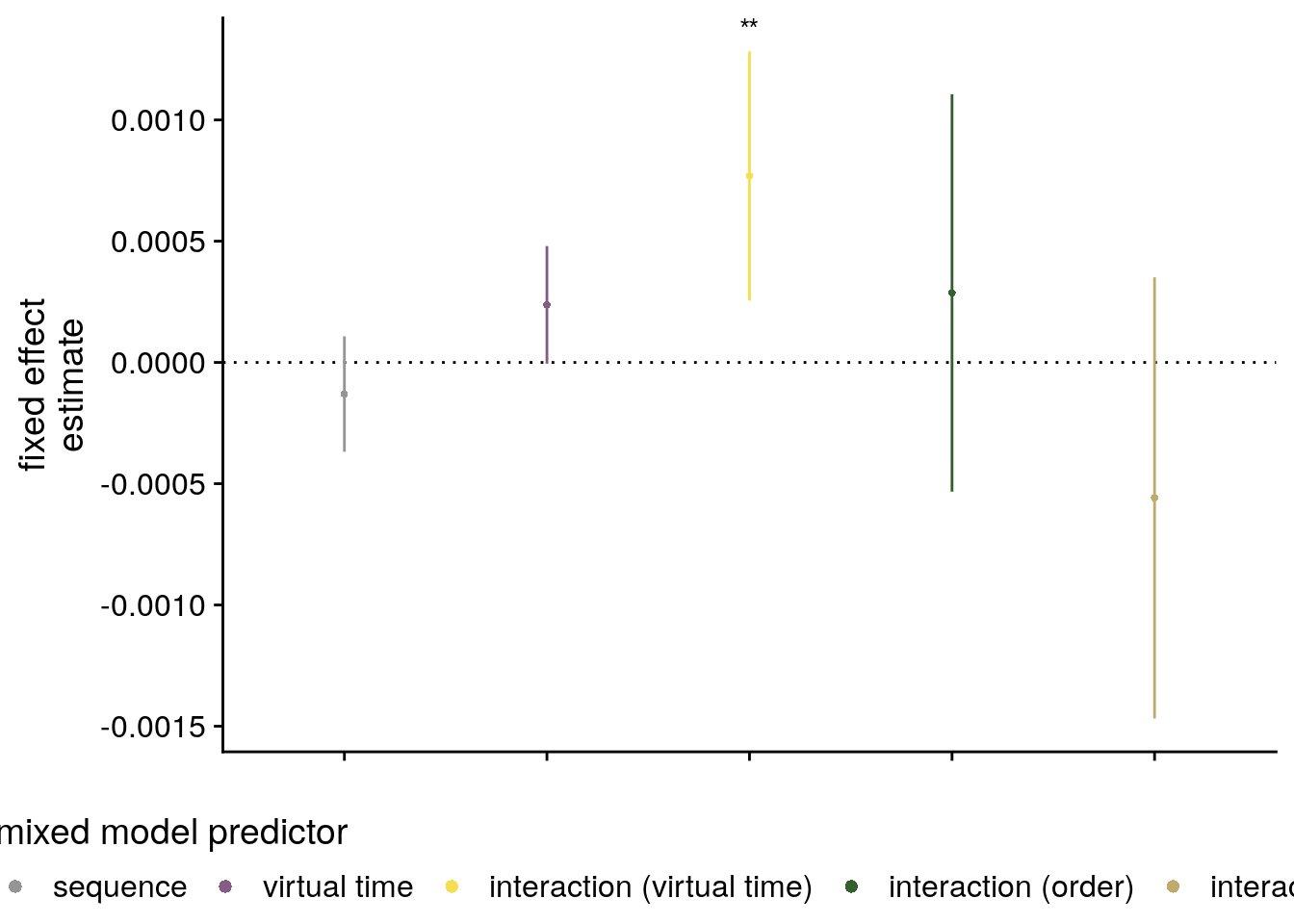
MDS
To explore how the event sequences could be arranged in a low-dimensional representational space, we want to run multi-dimensional scaling. To implement these analyses, we use the smacof-package, see also the helpful vignette here. MDS requires a distance matrix as an input. We will use a distance matrix based on the population-level predictions from the linear mixed model fitted to the anterior hippocampus pattern similarity change data as an input. This model captures the interaction between virtual temporal distances and sequence membership of event pairs on pattern similarity in the aHPC.
We first initialize a data frame that has one row for each possible pairwise comparison of two events and their (z-scored) absolute virtual temporal distances. We use this data frame as “new” data to predict pattern similarity changes from the linear mixed model. The resulting predicted pairwise similarity changes are converted to a matrix, converted to distances and scaled to the range from 0 to 1.
We aimed to explore how hippocampal event representations of the different sequences could be embedded in a low-dimensional representational space to give rise to the positive and negative correlations of pattern similarity change and temporal distances for same-sequence and different-sequence events, respectively. For each pair of events, we generated an expected similarity value (Supplemental Figure 6D) using the fixed effects of the mixed model fitted to hippocampal pattern similarity that captures the interaction between virtual temporal distances and sequence membership (c.f. Figure 5, Supplemental Figure 4IJ, and Supplemental Table 7). Using the predict-method implemented in the lme4-package109, we generated model-derived similarity values for all event pairs given their temporal distances and sequence membership. We chose this approach over the raw pattern similarity values to obtain less noisy estimates of the pairwise distances.
# check if virtual time exists
#(added for OSF code, which will not have this variable in the workspace yet because it did not run the design illustration script included in the full analysis)
if (!exists("virtual_time")){virtual_time <- beh_data %>% filter(sub_id=="31") %>% pull("virtual_time")} # virtual time is the same for all subjects
# create a tibble to use for MDS
# this tibble should have a row for each possible pairwise comparison of two events
mds_df <- expand_grid(virtual_time1=virtual_time, virtual_time2=virtual_time) %>%
mutate( # add design variables
day1 = rep(1:n_days, each=n_days*n_events_day^2),
day2 = rep(1:n_days, each=n_events_day, times=n_events_day*n_days),
event1 = rep(1:n_events_day, each=n_events_day*n_days, times=n_days),
event2 = rep(1:n_events_day, times=n_days^2*n_events_day),
idx1 = (day1-1)*5+event1, # for later conversion to matrix
ixd2 = (day2-1)*5+event2, # for later conversion to matrix
same_day = day1==day2,
same_day_dv = plyr::mapvalues(same_day, from = c(FALSE, TRUE), to = c(-1, 1)),
.before = virtual_time1) %>%
filter(!(day1==day2 & event1 == event2)) %>% # remove diagonal, important to do before z-scoring!
mutate(vir_time_diff = scale(abs(virtual_time1-virtual_time2))) # z-scored absolute virtual time difference
# for each event pair, get a predicted pattern similarity change value from the mixed model fitted to the aHPC data (ignoring the random effects)
mds_df$ps_change_hat <- predict(lmm_aHPC_interaction, newdata=mds_df, re.form=NA)
# turn into matrix (can probably be done in a prettier way without the loop)
ps_change_hat_mat <- matrix(0, nrow=n_events_day*n_days, ncol=n_events_day*n_days)
for (i in 1:nrow(mds_df)){
ps_change_hat_mat[mds_df$idx1[i], mds_df$ixd2[i]] <- mds_df$ps_change_hat[i]
}
# make plot of the resulting predicted pattern similarity change matrix
ps_change_hat_df <- reshape2::melt(ps_change_hat_mat)
f0a <- ggplot(ps_change_hat_df, aes(x=Var1, y=Var2, fill=value)) +
geom_tile() +
scale_y_reverse() +
scale_fill_scico(palette = "buda") +
ggtitle("predicted similarity change") +
xlab("events by day") +
ylab("events by day") +
labs(fill = "ps change") +
theme_cowplot() +
coord_fixed() #theme(aspect.ratio = 1)
# convert to distance matrix
ps_dist_hat_mat <- ps_change_hat_mat %>%
smacof::sim2diss(method = "corr")
# rescale from 0 to 1
ps_dist_hat_mat <- rescale(ps_dist_hat_mat, c(0,1))
diag(ps_dist_hat_mat)<-NA
# make plot of the resulting distance matrix
ps_dist_hat_df <- reshape2::melt(ps_dist_hat_mat)
f0b <- ggplot(ps_dist_hat_df, aes(x=Var1, y=Var2, fill=value)) +
geom_tile() +
scale_y_reverse() +
scale_fill_scico(palette = "buda", limits=c(0,1)) +
theme_cowplot() +
coord_fixed()+ #theme(aspect.ratio = 1) +
ggtitle("corresponding distance matrix") +
xlab("events by day") +
ylab("events by day") +
labs(fill = "distance")
f0a +f0b &
plot_annotation(tag_levels = 'A',
title = "MDS based on mixed model fitted to aHPC pattern similarity change") &
theme(text = element_text(size=10, family = font2use),
axis.text = element_text(size=8),
legend.text=element_text(size=8),
legend.title=element_text(size=8),
legend.position = 'right',
plot.tag = element_text(size = 10))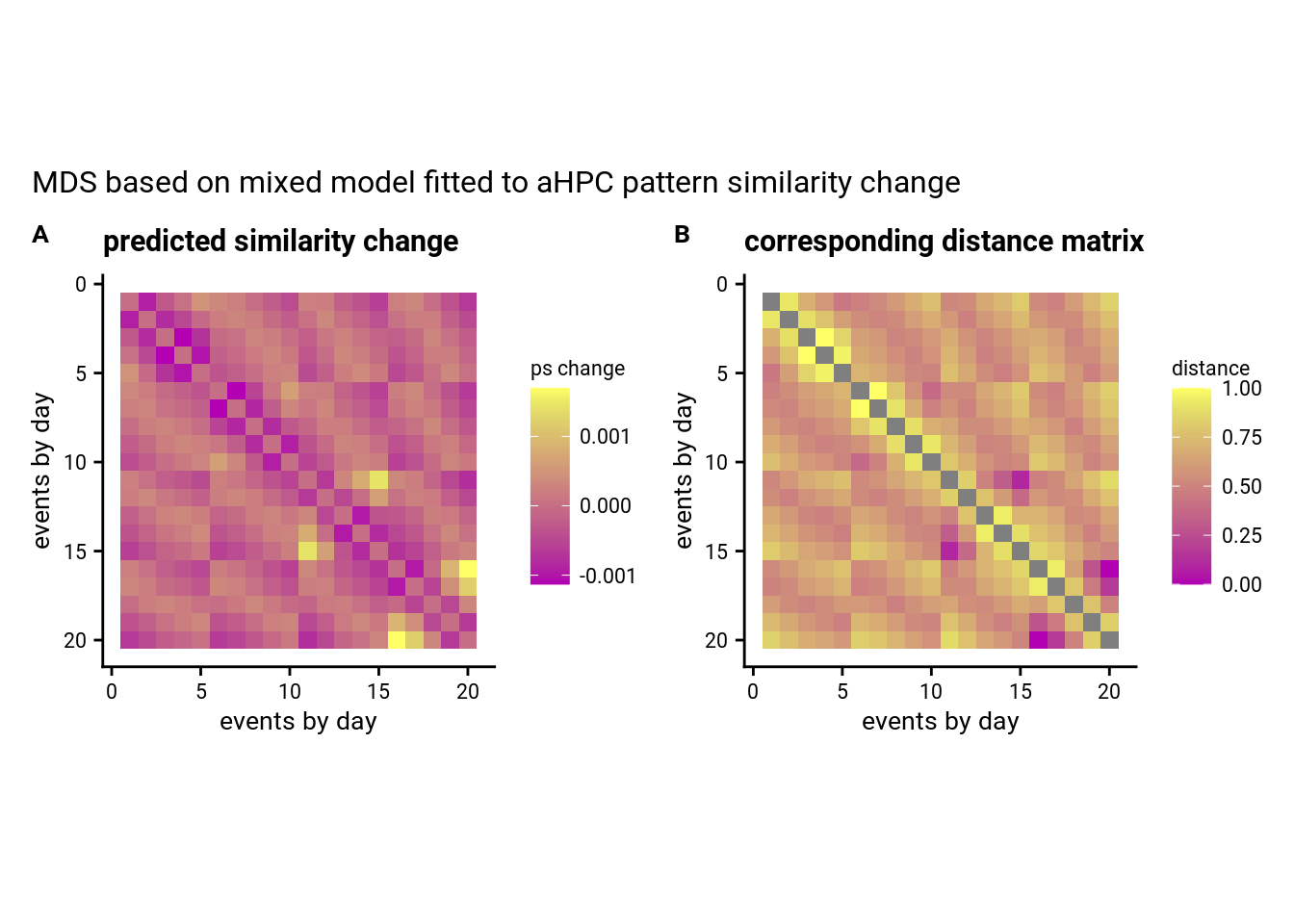
# make plot of lower triangle only of the resulting distance matrix
lt <- upper.tri(ps_dist_hat_mat, diag = TRUE)
lt_df <- reshape2::melt(lt)
ps_dist_hat_df <- reshape2::melt(ps_dist_hat_mat)
ps_dist_hat_df<-ps_dist_hat_df[lt_df$value,]
sfig_mds_input <- ggplot(ps_dist_hat_df, aes(x=Var1, y=Var2, fill=value)) +
geom_tile() +
scale_y_reverse() +
scale_fill_scico(palette = "buda", limits=c(0,1), breaks=c(0,1)) +
theme_cowplot() +
coord_fixed() +
xlab("events by sequence") +
ylab("events by sequence") +
guides(fill=guide_colorbar(title="distance", title.hjust = 1, barwidth = 0.3, barheight = 0.7)) +
theme(text = element_text(size=6, family = font2use),
axis.text = element_text(size=6),
legend.text=element_text(size=6),
legend.title=element_text(size=6),
legend.position = c(1,1), legend.justification = c(1,1))
sfig_mds_input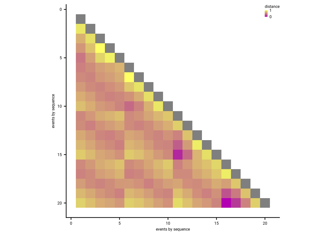
# save and print
fn <- here("figures", "mds_input_mat")
ggsave(paste0(fn, ".pdf"), plot=sfig_mds_input, units = "cm",
width = 3, height = 3, dpi = "retina", device = cairo_pdf)
ggsave(paste0(fn, ".png"), plot=sfig_mds_input, units = "cm",
width = 3, height = 3, dpi = "retina", device = "png")We are now ready to run MDS. We subject the distance matrix to MDS using an ordinal model (i.e. non-metric MDS) using two dimensions. Because MDS is sensitive to the starting configuration, we run MDS many times using random starting configurations. From the resulting configurations, we pick the one resulting in the lowest stress. This procedure is described in the vignette of the smacof-package, which we use for these analyses.
Using the smacof-package111, the model-predicted similarities were converted to distances and the resulting distance matrix (Supplemental Figure 6D) was subjected to non-metric multidimensional scaling using two dimensions. We chose two dimensions to be able to intuitively visualize the results. Because MDS is sensitive to starting values, we ran multidimensional scaling 1000 times with random initial configurations and visualized the resulting configuration with the lowest stress value. Basing this analysis on the model-derived similarities assumes the same relationship of virtual temporal distances for all event pairs from different sequences, but we would like to note that not all solutions we observed, in particular those with higher stress values, resulted in parallel configurations for the four sequences.
Metric MDS
Let’s begin by testing out MDS using a ratio transformation.
# because MDS is sensitive to the start configuration, let's run it with many different random configurations (take the best in the end)
n_rand_starts <- 1000
# maximum number of iterations
max_it <- 5000
# run MDS for 2 dimensions n_rand_starts times with random start configuration and store best fit
set.seed(106) # set seed for reproducibility
stressvec <- rep(NA, n_rand_starts)
fitbest <- mds(ps_dist_hat_mat, ndim = 2, itmax = max_it, init = "random", type = "ratio")
stressvec[1] <- fitbest$stress
for(i in 2:n_rand_starts) {
fitran <- mds(ps_dist_hat_mat, ndim = 2, itmax = max_it, init = "random", type = "ratio")
stressvec[i] <- fitran$stress
if (fitran$stress < fitbest$stress){
fitbest <- fitran}
}
# get data frame of resulting configuration
conf <- as.data.frame(fitbest$conf)
conf$day <- factor(rep(1:n_days, each = n_events_day))
conf$event <- factor(rep(1:n_events_day,n_days))
conf$virtual_time <- virtual_time
# visualize as 2D scatter with lines of the configuration
ratioMDS_confplot <- ggplot(conf, aes(x=D1,y=D2, group=day, color=virtual_time, fill=virtual_time, shape=event)) +
geom_path(aes(linetype=day),size=0.5, color="grey") +
scale_linetype_manual(values=c("solid", "dashed", "dotted", "3111")) +
geom_point(size=2) +
scale_shape_manual(values = c(21:25)) +
scico::scale_fill_scico(begin = 0.1, end = 0.7, palette = "devon", breaks=c(8,22)) +
scico::scale_color_scico(begin = 0.1, end = 0.7, palette = "devon") +
guides(linetype=guide_legend(title = "sequence", title.position="top", title.hjust = 0.5, order=3),
shape=guide_legend(override.aes = list(shape = c(21:25), color = NA, fill = "grey"), title.position="top", title.hjust = 0.5, order=2),
fill=guide_colorbar(title="virtual time", title.position="top", title.hjust = 1, barwidth = 2, barheight = 0.5, order=1),
color= "none"
) +
xlab("dimension 1") +
ylab("dimension 2") +
theme_cowplot() +
coord_fixed() +
theme(#aspect.ratio = 1,
legend.spacing.x = unit(1, 'mm'),
legend.key.size = unit(2.5,"mm"),
#legend.margin = margin(0,0,0,0.5, unit="cm"),
legend.position = "right",
legend.justification = "left")
ratioMDS_confplot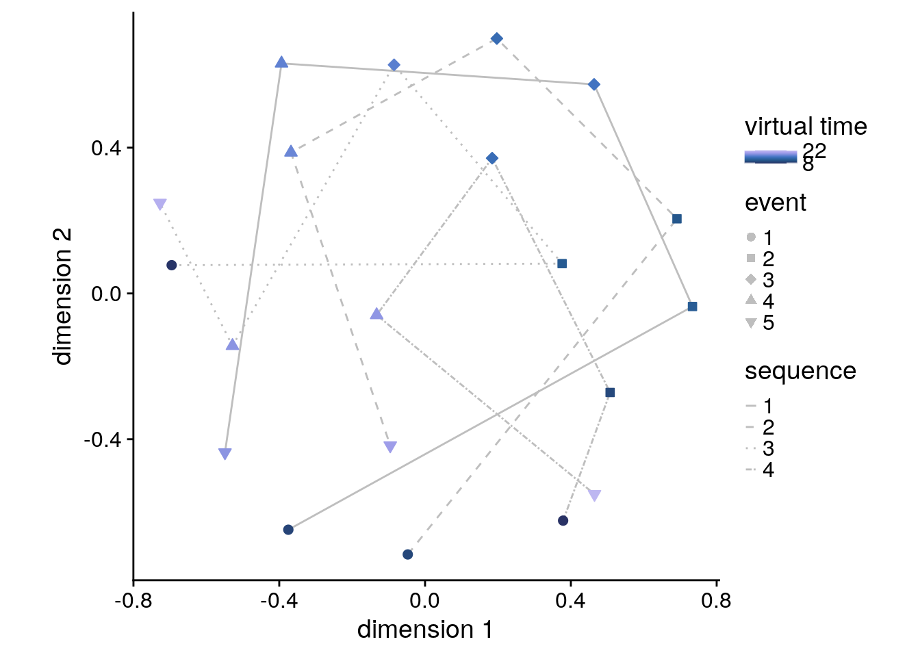
Let’s test how good this fit really is. As described in the smacof-vignette, one way to do so is to run a permutation test to compare the observed stress value against a surrogate distribution generated from applying MDS to a shuffled distance matrix. To visualize the result, we plot a histogram of the permutation distribution as well as the critical (5th percentile) and the observed stress value.
# permutation test to assess fit relative to permuted data
set.seed(107) # set seed for reproducibility
perm_fitbest <- permtest(fitbest, nrep = 1000, verbose = FALSE)
perm_fitbest##
## Call: permtest.smacof(object = fitbest, nrep = 1000, verbose = FALSE)
##
## SMACOF Permutation Test
## Number of objects: 20
## Number of replications (permutations): 1000
##
## Observed stress value: 0.366
## p-value: 0.999# get p and z-value
p_perm <- sum(c(perm_fitbest$stress.obs, perm_fitbest$stressvec) <= perm_fitbest$stress.obs)/(perm_fitbest$nrep+1)
z_perm <- (perm_fitbest$stress.obs-mean(perm_fitbest$stressvec))/sd(perm_fitbest$stressvec)
# plot of permutation test results
perm_fitbest_df <- tibble(stress_perms = perm_fitbest$stressvec)
prctile <- as.character(expression(95^{th}*" percentile"))
ratioMDS_permplot <- ggplot(perm_fitbest_df, aes(x=stress_perms)) +
geom_histogram(aes(y=stat(width*density)), bins = 50, fill = ultimate_gray) +
geom_segment(aes(x = perm_fitbest$stress.obs, y = 0, xend = perm_fitbest$stress.obs, yend = 0.02),
color="#972D15") +
geom_segment(aes(x = quantile(stress_perms, 0.05), y = 0,
xend = quantile(stress_perms, 0.05), yend = 0.04),
color="Black", linetype="dashed") +
geom_label(aes(x=quantile(stress_perms, probs=0.05), y=0.04, label = prctile),
hjust=0, vjust=0, size=6/.pt, fill = "white", alpha=0.5, color="BLACK", parse = TRUE,
label.padding = unit(0.1, "lines"), label.size = 1/.pt,) +
geom_label(aes(x=perm_fitbest$stress.obs, y=0.02, label="observed stress"),
label.padding = unit(0.1, "lines"), label.size = 1/.pt,
hjust=1, vjust=0.5, size=6/.pt, fill = "white", alpha=0.5, color="#972D15") +
scale_y_continuous(labels = scales::percent) +
ylab("% of shuffles") +
xlab("stress (null distr.)") +
theme_cowplot() +
theme(legend.position = "none", text = element_text(size=10, family=font2use),
axis.text = element_text(size=8),
legend.text=element_text(size=8),
legend.title=element_text(size=8))
ratioMDS_permplot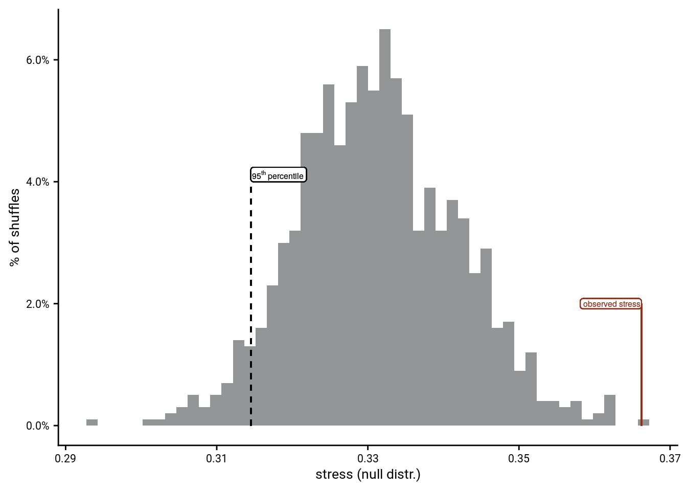
Permutation test of observed stress against shuffles for metric (ratio) MDS: z=3.3, p=0.999
Non-metric MDS
Because the permutation test is not significant for metric MDS, we continue with non-metric MDS.
# because MDS is sensitive to the start configuration, let's run it with many different random configurations (take the best in the end)
n_rand_starts <- 1000
# maximum number of iterations
max_it <- 5000
# run MDS for 2 dimensions n_rand_starts times with random start configuration and store best fit
set.seed(106) # set seed for reproducibility
stressvec <- rep(NA, n_rand_starts)
fitbest <- mds(ps_dist_hat_mat, ndim = 2, itmax = max_it, init = "random", type = "ordinal")
stressvec[1] <- fitbest$stress
for(i in 2:n_rand_starts) {
fitran <- mds(ps_dist_hat_mat, ndim = 2, itmax = max_it, init = "random", type = "ordinal")
stressvec[i] <- fitran$stress
if (fitran$stress < fitbest$stress){
fitbest <- fitran}
}
# get data frame of resulting configuration
conf <- as.data.frame(fitbest$conf)
conf$day <- factor(rep(1:n_days, each = n_events_day))
conf$event <- factor(rep(1:n_events_day,n_days))
conf$virtual_time <- virtual_time
# visualize as 2D scatter with lines of the configuration
f5c <- ggplot(conf, aes(x=D1,y=D2, group=day, color=virtual_time, fill=virtual_time, shape=event)) +
geom_path(aes(linetype=day),size=0.5, color="grey") +
scale_linetype_manual(values=c("solid", "dashed", "dotted", "3111")) +
geom_point(size=2) +
scale_shape_manual(values = c(21:25)) +
scico::scale_fill_scico(begin = 0.1, end = 0.7, palette = "devon", breaks=c(8,22)) +
scico::scale_color_scico(begin = 0.1, end = 0.7, palette = "devon") +
guides(linetype=guide_legend(title = "sequence", title.position="top", title.hjust = 0.5, order=3),
shape=guide_legend(override.aes = list(shape = c(21:25), color = NA, fill = "grey"), title.position="top", title.hjust = 0.5, order=2),
fill=guide_colorbar(title="virtual time", title.position="top", title.hjust = 1, barwidth = 2, barheight = 0.5, order=1),
color= "none"
) +
xlab("dimension 1") +
ylab("dimension 2") +
theme_cowplot() +
coord_fixed() +
theme(#aspect.ratio = 1,
legend.spacing.x = unit(1, 'mm'),
legend.key.size = unit(2.5,"mm"),
#legend.margin = margin(0,0,0,0.5, unit="cm"),
legend.position = "right",
legend.justification = "left")
f5c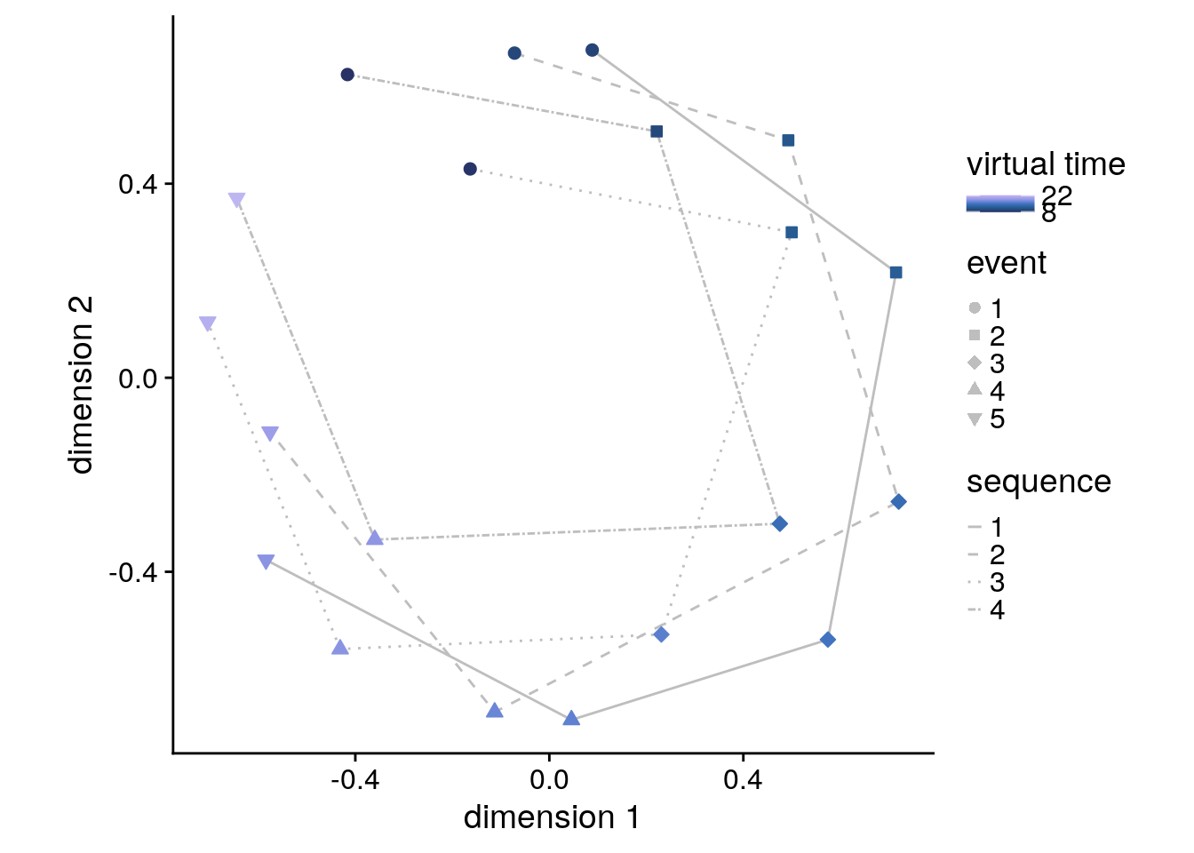
# save source data
source_dat <-ggplot_build(f5c)$data[[2]]
readr::write_tsv(source_dat %>% select(x, y, colour, group, shape),
file = file.path(dirs$source_dat_dir, "f5c.txt"))
#comparing metric and non-metric MDS
mds_fig <- f5c + ratioMDS_confplot +
plot_layout(guides = "collect") &
theme(text = element_text(size=10, family = font2use),
axis.text = element_text(size=8),
legend.text=element_text(size=8),
legend.title=element_text(size=8),
plot.tag = element_text(size = 10)) &
plot_annotation(tag_levels = 'A')
mds_fig[[1]] <- mds_fig[[1]] + ggtitle("non-metric MDS")
mds_fig[[2]] <- mds_fig[[2]] + ggtitle("metric MDS")
mds_fig <- mds_fig &
theme(text = element_text(size=10, family = font2use),
axis.text = element_text(size=8),
legend.text=element_text(size=8),
legend.title=element_text(size=8),
plot.tag = element_text(size = 10),
legend.position = "bottom") &
plot_annotation(tag_levels = 'A')
# save and print (height was 18 when incl. searchlights)
fn <- here("figures", "mds_fig")
ggsave(paste0(fn, ".png"), plot=mds_fig, units = "cm",
width = 14.4, height = 10, dpi = "retina", device = "png")
mds_fig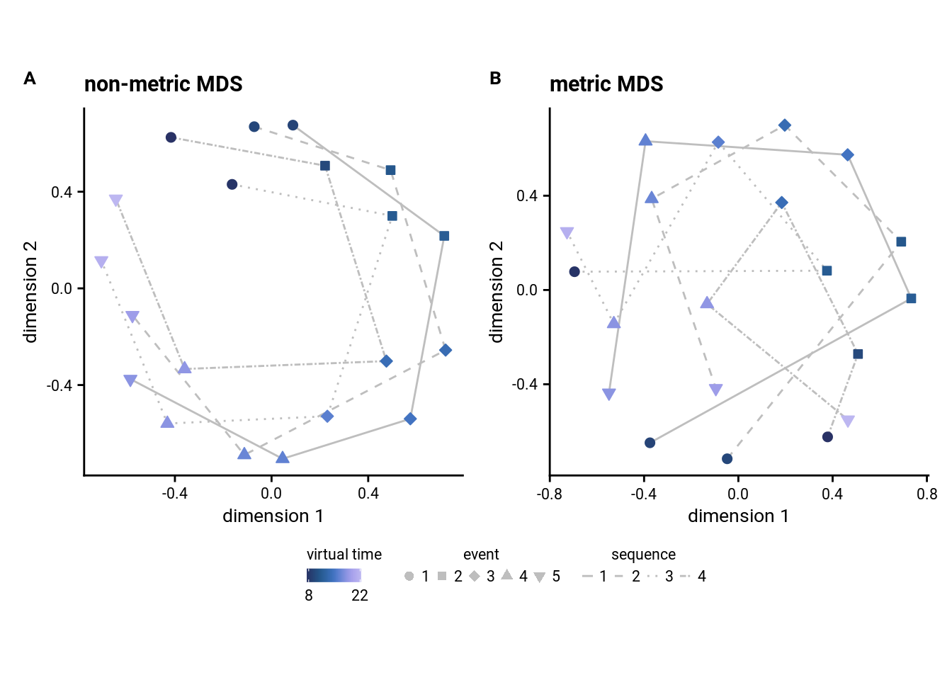
Let’s test how good the non-metric fit really is. As described in the smacof-vignette, one way to do so is to run a permutation test to compare the observed stress value against a surrogate distribution generated from applying MDS to a shuffled distance matrix. To visualize the result, we plot a histogram of the permutation distribution as well as the critical (5th percentile) and the observed stress value.
We tested the stress value of the resulting configuration against a surrogate distribution of stress values obtained from permuting the input distances on each of 1000 iterations. Using the mean and standard deviation of the resulting null distribution, we obtained a z-value as a test statistic and report the proportion of stress values in the null distribution that were equal to or smaller than the observed stress value (Supplemental Figure 6E).
# permutation test to assess fit relative to permuted data
set.seed(107) # set seed for reproducibility
perm_fitbest <- permtest(fitbest, nrep = 1000, verbose = FALSE)
perm_fitbest##
## Call: permtest.smacof(object = fitbest, nrep = 1000, verbose = FALSE)
##
## SMACOF Permutation Test
## Number of objects: 20
## Number of replications (permutations): 1000
##
## Observed stress value: 0.261
## p-value: <0.001# get p and z-value
p_perm <- sum(c(perm_fitbest$stress.obs, perm_fitbest$stressvec) <= perm_fitbest$stress.obs)/(perm_fitbest$nrep+1)
z_perm <- (perm_fitbest$stress.obs-mean(perm_fitbest$stressvec))/sd(perm_fitbest$stressvec)
# plot of permutation test results
perm_fitbest_df <- tibble(stress_perms = perm_fitbest$stressvec)
prctile <- as.character(expression(95^{th}*" percentile"))
sfig6_e <- ggplot(perm_fitbest_df, aes(x=stress_perms)) +
geom_histogram(aes(y=stat(width*density)), bins = 50, fill = ultimate_gray) +
geom_segment(aes(x = perm_fitbest$stress.obs, y = 0, xend = perm_fitbest$stress.obs, yend = 0.02),
color="#972D15") +
geom_segment(aes(x = quantile(stress_perms, 0.05), y = 0,
xend = quantile(stress_perms, 0.05), yend = 0.04),
color="Black", linetype="dashed") +
geom_label(aes(x=quantile(stress_perms, probs=0.05), y=0.04, label = prctile),
hjust=0, vjust=0, size=6/.pt, fill = "white", alpha=0.5, color="BLACK", parse = TRUE,
label.padding = unit(0.1, "lines"), label.size = 1/.pt,) +
geom_label(aes(x=perm_fitbest$stress.obs, y=0.02, label="observed stress"),
label.padding = unit(0.1, "lines"), label.size = 1/.pt,
hjust=0, vjust=0.5, size=6/.pt, fill = "white", alpha=0.5, color="#972D15") +
scale_y_continuous(labels = scales::percent) +
ylab("% of shuffles") +
xlab("stress (null distr.)") +
theme_cowplot() +
theme(legend.position = "none", text = element_text(size=10, family=font2use),
axis.text = element_text(size=8),
legend.text=element_text(size=8),
legend.title=element_text(size=8))
sfig6_e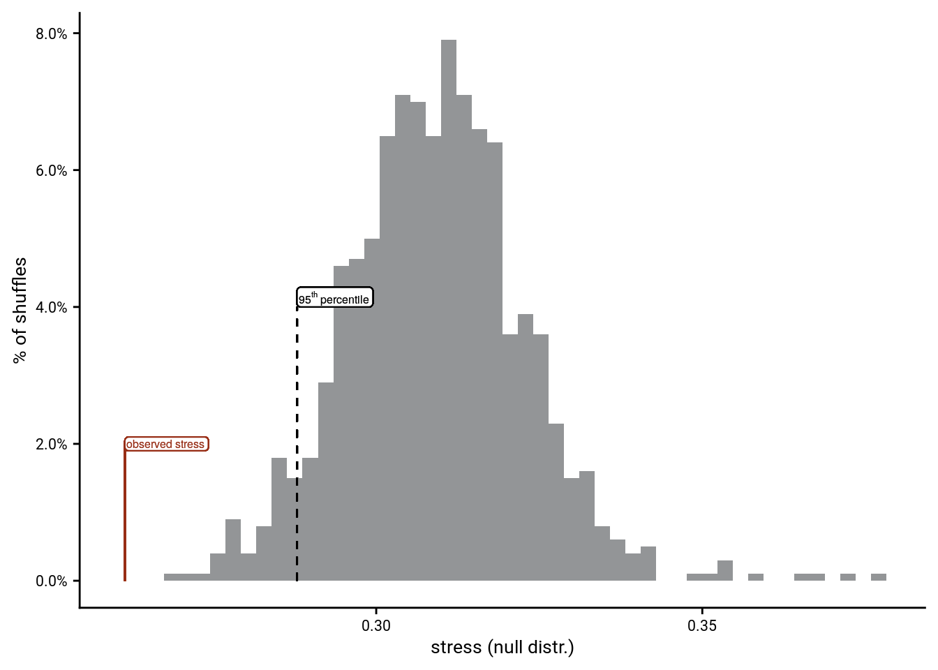
Permutation test of observed stress against shuffles for non-metric (ordinal) MDS: z=-3.5, p=0.001
To test whether the resulting configuration exhibits higher distances between pairs of events that have a high input distance we run a t-test for independent samples based on a median split (high vs. low input distance).
# create dataframe that includes event and MDS configuration information
idx_mat <- matrix(TRUE, nrow=20, ncol=20)
fit_best_df<- tibble(day1 = day[which(lower.tri(idx_mat), arr.ind = TRUE)[,"row"]],
day2 = day[which(lower.tri(idx_mat), arr.ind = TRUE)[,"col"]],
event1 = event[which(lower.tri(idx_mat), arr.ind = TRUE)[,"row"]],
event2 = event[which(lower.tri(idx_mat), arr.ind = TRUE)[,"col"]],
delta = as.numeric(fitbest$delta),
confdist = as.numeric(fitbest$confdist),
same_day = day1 == day2)
# median split variable based on input distances (delta)
fit_best_df <- fit_best_df %>%
mutate(high_low = sjmisc::dicho(fit_best_df$delta),
high_low_f = factor(if_else(high_low ==1, "high", "low")))
# do t-test based on median split
stats <- fit_best_df %>%
do(tidy(t.test(confdist ~ high_low_f, data = ., var.equal = TRUE)))
# Cohen's d with Hedges' correction for independent samples
d<-cohen.d(d = fit_best_df%>%filter(high_low_f == "high") %>% pull(confdist),
f = fit_best_df%>%filter(high_low_f == "low") %>% pull(confdist),
paired=FALSE, hedges.correction=TRUE, noncentral=FALSE)
stats$d <- d$estimate
stats$dCI_low <- d$conf.int[[1]]
stats$dCI_high <- d$conf.int[[2]]
huxtable(stats) %>% theme_article()| estimate | estimate1 | estimate2 | statistic | p.value | parameter | conf.low | conf.high | method | alternative | d | dCI_low | dCI_high |
|---|---|---|---|---|---|---|---|---|---|---|---|---|
| 0.419 | 1.1 | 0.683 | 9.35 | 2.71e-17 | 188 | 0.331 | 0.507 | Two Sample t-test | two.sided | 1.35 | 1.03 | 1.67 |
sfig6_f <- ggplot(fit_best_df, aes(x=high_low, y=confdist, fill=high_low, color=high_low)) +
geom_boxplot(width = .1, colour = "black", outlier.shape = NA, outlier.size = 2) +
gghalves::geom_half_violin(data=fit_best_df %>% filter(high_low==0), aes(x=1, y=confdist),
position=position_nudge(-0.1), side = "l", colour=NA) +
gghalves::geom_half_violin(data=fit_best_df %>% filter(high_low==1), aes(x=2, y=confdist),
position=position_nudge(0.1), side = "r", colour=NA) +
geom_point(aes(x=ifelse(high_low==0, 1.2, 1.8)), alpha = 1, position = position_jitter(width = .1, height = 0), shape = 16, size = 1) +
stat_summary(fun = mean, geom = "point", size=1, shape = 16,
position = position_nudge(c(-0.1, 0.1)), colour = "BLACK") +
stat_summary(fun.data = mean_se, geom = "errorbar",
position = position_nudge(c(-0.1, 0.1)), colour = "BLACK", width = 0, size = 0.5) +
ylab('MDS distance')+xlab('input distance') +
annotate(geom = "text", x = 1.5, y = Inf, label = 'underline(" *** ")',
hjust = 0.5, vjust=1, size = 8/.pt, family=font2use, parse=TRUE) +
scale_x_discrete(labels = c("low", "high")) +
scale_color_manual(values=c("lightgrey", "darkgrey"), labels=c("low", "high")) +
scale_fill_manual(values=c("lightgrey", "darkgrey")) +
guides(color=guide_legend("input distance", override.aes = list(shape=16, size=1, linetype=0, fill=NA, alpha=1)), fill = "none") +
theme_cowplot() +
theme(legend.position = "none", text = element_text(size=10, family=font2use),
axis.text = element_text(size=8),
legend.text=element_text(size=8),
legend.title=element_text(size=8))
sfig6_f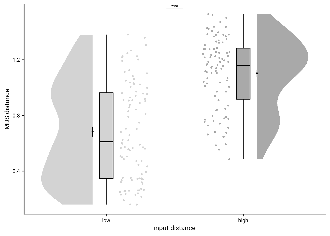
Summary Statistics: t-test of resulting MDS distances contrasting event pairs separated by high vs. low input distances (median split): t188=9.35, p=0.000, d=1.35, 95% CI [1.03, 1.67]
Additionally, we contrasted the distances between pairs of events in the resulting configuration between distances separated by high or low (median split) input distances using a t-test for independent samples (Supplemental Figure 6F). Using a Spearman correlation, we quantified the relationship of the input distances and the distances in the resulting configuration (Supplemental Figure 6G).
To further assess the fit of the configuration to the underlying distance matrix, we calculate the correlation between input distances between event pairs and the distances in the resulting MDS configuration as well as conducting a permutation test to assess the resulting stress value.
# correlate input distances and configuration distances
stats <- tidy(cor.test(fit_best_df$delta, fit_best_df$confdist, method = "spearman"))## Warning in cor.test.default(fit_best_df$delta, fit_best_df$confdist, method = "spearman"): Cannot compute exact p-value with ties# Shepard plot showing input distances and configuration distances
sfig6_g <- ggplot(fit_best_df,aes(x = rank(delta), y = rank(confdist))) +
geom_point(size = 0.5) +
geom_smooth(method = "lm", formula = "y ~ x", color = "darkgrey") +
#annotate("text", x=Inf, y=-Inf, hjust="inward", vjust="inward", size=6/.pt,
# label=sprintf("r=%.2f\np=%.3f", round(stats$estimate, digits=2), round(stats$p.value, digits=3)),
# family=font2use) +
xlab("input distance") +
ylab("MDS distance") +
theme_cowplot()
sfig6_g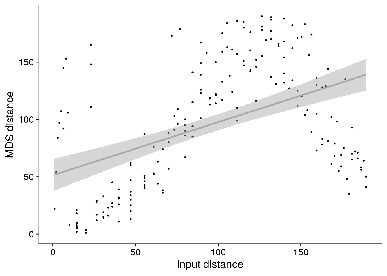 Spearman correlation of input distances and distances in resulting MDS configuration:
r=0.46, p=0.000
We are ready to create figure 5:
# start figure 5 by making the MDS plot
layout = "
A
A
B"
f5c_guide <- f5c / guide_area() +
plot_layout(design =layout, guides = "collect") &
theme(legend.direction = "horizontal",
legend.box = "vertical",
text = element_text(size=10, family = font2use),
axis.text = element_text(size=8),
legend.text=element_text(size=8),
legend.title=element_text(size=8),
plot.tag = element_text(size = 10))
# add the three panels together
layout = "ABC"
f5 <- f5a + f5b + f5c_guide +
plot_layout(guides = "keep", design = layout) &
theme(text = element_text(size=10, family = font2use),
axis.text = element_text(size=8),
legend.text=element_text(size=8),
legend.title=element_text(size=8),
plot.tag = element_text(size = 10)) &
plot_annotation(tag_levels = 'A')
# save and print (height was 18 when incl. searchlights)
fn <- here("figures", "f5")
ggsave(paste0(fn, ".pdf"), plot=f5, units = "cm",
width = 18, height = 10, dpi = "retina", device = cairo_pdf)
ggsave(paste0(fn, ".png"), plot=f5, units = "cm",
width = 18, height = 10, dpi = "retina", device = "png")
Figure 5. The anterior hippocampus generalizes temporal relations across sequences. A. Z-values show results of participant-specific linear models quantifying the effect of virtual time for event pairs from the same sequence (blue, as in Figure 4B) and from different sequences (red). Temporal distance is negatively related to hippocampal representational change for event pairs from different sequences. See Supplemental Figure 4EF for mixed model analysis of across-sequence comparisons. The effect of virtual time differs for comparisons within the same sequence or between two different sequences. B. To illustrate the effect shown in A, average pattern similarity change values are shown for across–sequence event pairs that are separated by low and high temporal distances based on a median split. C. Multidimensional scaling results show low-dimensional embedding of the event sequences. Shapes indicate event order, color shows virtual times of events. The different lines connect the events belonging to the four sequences for illustration. *** p≤0.001; ** p<0.01; * p<0.05
UMAP
To check if the MDS results depend on the specific algorithm, let’s also try the UMAP (Uniform Manifold Approximation and Projection for Dimension Reduction) algorithm on the mixed model distance matrix.
# set up umap config based on defaults, but using distance matrix as input and define the two parameters
custom_config = umap.defaults
custom_config$input = "dist"
custom_config$n_neighbors <- 6 # k nearest neighbors: high-values push towards global structure at cost of detail
custom_config$min_dist <- 0.1 # minimum distance: high values lead to looser packing, but better topology
# run umap using the LME distance matrix as input. use the custom config
set.seed(306) # set seed for reproducibility
umap_dist = umap(ps_dist_hat_mat, config = custom_config)
# turn this solution into a tibble and include info about days and events
umap_df <- tibble(day = factor(rep(c(1:n_days), each=n_events_day)),
event = factor(rep(1:n_events_day,n_days)),
virtual_time <- virtual_time,
umapX = umap_dist$layout[,1],
umapY = umap_dist$layout[,2])
# visualize as 2D scatter with lines of the configuration
sfig6_x <- ggplot(umap_df, aes(x=umapX,y=umapY, group=day, color=virtual_time, fill=virtual_time, shape=event)) +
geom_path(aes(linetype=day),size=0.5, color="grey") +
scale_linetype_manual(values=c("solid", "dashed", "dotted", "3111")) +
geom_point(size=2) +
scale_shape_manual(values = c(21:25)) +
scico::scale_fill_scico(begin = 0.1, end = 0.7, palette = "devon", breaks=c(8,22)) +
scico::scale_color_scico(begin = 0.1, end = 0.7, palette = "devon") +
guides(linetype = guide_legend(title = "sequence", title.position="top", title.hjust = 0.5, order=1),
shape = guide_legend(override.aes = list(shape = c(21:25), color = NA, fill = "grey"), title.position="top", title.hjust = 0.5, order=2),
fill = guide_colorbar(title="virtual time", title.position="top", title.hjust = 1, barwidth = 0.5, barheight = 1),
color = "none"
) +
xlab("dimension 1") +
ylab("dimension 2") +
theme_cowplot() +
coord_fixed() +
theme(legend.spacing.x = unit(1, 'mm'),
legend.key.size = unit(2.5,"mm"),
legend.position = "right",
legend.justification = "left")
sfig6_x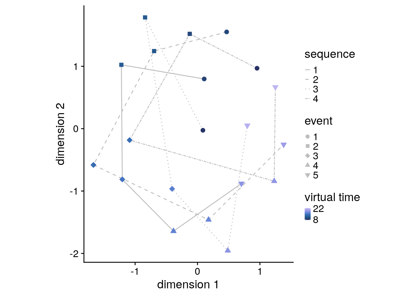
Let’s create supplemental figure 6
layout = "
AADDFF
AADDFF
BCEEGG"
sfig6 <- sfig6_a + sfig6_b + sfig6_c + plot_spacer() + sfig6_e + sfig6_f + sfig6_g +
plot_layout(design = layout, guides = "collect") +
plot_annotation(theme = theme(plot.margin = margin(t=0, r=0, b=0, l=0, unit="cm")),
tag_levels = list(c('A', 'B', 'C', 'E', 'F', 'G'))) &
theme(text = element_text(size=10, family = font2use),
axis.text = element_text(size=8),
legend.position = 'bottom',
plot.tag = element_text(size = 10),
legend.margin=margin(r = 0, unit='cm'))
fn <- here("figures", "sf06")
ggsave(paste0(fn, ".pdf"), plot=sfig6, units = "cm",
width = 17.4, height = 12, dpi = "retina", device = cairo_pdf)
ggsave(paste0(fn, ".png"), plot=sfig6, units = "cm",
width = 17.4, height = 12, dpi = "retina", device = "png")
Supplemental Figure 6. Virtual time predicts hippocampal pattern similarity change for events from different sequences. A. Z-values show the relationship of the different time metrics to representational change in the anterior hippocampus based on participant-specific multiple regression analyses for pairs of events from different sequences. Circles show participant-specific Z-values from summary statistics approach; boxplot shows median and upper/lower quartile along with whiskers extending to most extreme data point within 1.5 interquartile ranges above/below the upper/lower quartile; black circle with error bars corresponds to mean±S.E.M.; distribution shows probability density function of data points. B, C. Parameter estimates with 95% CIs (B) and estimated marginal means (C) show the fixed effects of the three time metrics from the corresponding mixed model. * p<0.05 after exclusion of one outlier excluded based on the boxplot criterion. D. A linear mixed model capturing the interaction effect of virtual temporal distances and sequence membership (Figure 5, Supplemental Figure 4IJ) was fitted to hippocampal representational change. An event-by-event similarity matrix was derived from the fixed effects of this model. Similarities were converted distances and then used as input for multidimensional scaling (see Methods). E. The stress value observed in the MDS analysis (red line) was significantly smaller than the 5th percentile (black dashed line) of a surrogate distribution of stress values obtained from shuffling the dissimilarities before running MDS in each of 1000 iterations. F. Pairs of events separated by a large distance in the input distance matrix were separated by a larger Euclidean distance in the resulting MDS configuration (t188=9.35, p<0.001, d=1.35, 95% CI [1.03, 1.67]). *** p <0.001. G. There was a significant Spearman correlation of input distances and MDS configuration distances (r=0.46, p<0.001), but visual inspection reveals a non-linear relationship where very high distances are systematically underestimated in the MDS configuration. This is likely because the data were projected onto only two dimensions for visualization. More dimensions would be needed to improve the fit of the MDS configuration and the input distance matrix. Distances are shown as ranks because non-metric MDS was used (high ranks for high distances).
8.9 alEC
So far we focused on the anterior hippocampus. But what about our second region of interest, the anterior-lateral entorhinal cortex (alEC)?
alEC: virtual time within/across sequences separately
First, we run the t-tests against zero for the alEC, separately for events from the same or two different sequences.
set.seed(108) # set seed for reproducibility
# run a group-level t-test on the RSA fits from the first level in alEC for within-day
stats <- rsa_fit %>%
filter(roi == "alEC_lr", same_day == TRUE) %>%
select(z_virtual_time) %>%
paired_t_perm_jb (., n_perm = n_perm)
# print results
huxtable(stats) %>% theme_article()| estimate | statistic | p.value | p_perm | parameter | conf.low | conf.high | method | alternative |
|---|---|---|---|---|---|---|---|---|
| -0.233 | -1.26 | 0.217 | 0.215 | 27 | -0.611 | 0.145 | One Sample t-test | two.sided |
# re-run without outliers (see outliers in subsequent plot)
alEC_within <- rsa_fit %>%
filter(roi == "alEC_lr", same_day == TRUE)
# find outliers
is_outlier <- function(x) {
return(x < quantile(x, 0.25) - 1.5 * IQR(x) | x > quantile(x, 0.75) + 1.5 * IQR(x))
}
out_ind <- is_outlier(alEC_within$z_virtual_time)
# run second-level analysis on data points that are not outliers
set.seed(123) # set seed for reproducibility
stats <- alEC_within[!out_ind,] %>%
select(z_virtual_time) %>%
paired_t_perm_jb (., n_perm = n_perm)
# Cohen's d with Hedges' correction for one sample using non-central t-distribution for CI
d<-cohen.d(d=alEC_within[!out_ind,]$z_virtual_time,
f=NA, paired=TRUE, hedges.correction=TRUE, noncentral=TRUE)
stats$d <- d$estimate
stats$dCI_low <- d$conf.int[[1]]
stats$dCI_high <- d$conf.int[[2]]
huxtable(stats) %>% theme_article()| estimate | statistic | p.value | p_perm | parameter | conf.low | conf.high | method | alternative | d | dCI_low | dCI_high |
|---|---|---|---|---|---|---|---|---|---|---|---|
| -0.482 | -3.54 | 0.00166 | 0.002 | 24 | -0.763 | -0.201 | One Sample t-test | two.sided | -0.685 | -1.17 | -0.268 |
Summary Statistics: t-test against 0 for virtual time within sequence in alEC (outliers excluded)
t24=-3.54, p=0.002, d=-0.69, 95% CI [-1.17, -0.27]
# run a group-level t-test on the RSA fits from the first level in alEC for across-day
set.seed(145) # set seed for reproducibility
stats <- rsa_fit %>%
filter(roi == "alEC_lr", same_day == FALSE) %>%
select(z_virtual_time) %>%
paired_t_perm_jb (., n_perm = n_perm)
# Cohen's d with Hedges' correction for one sample using non-central t-distribution for CI
d<-cohen.d(d=(rsa_fit %>% filter(roi == "alEC_lr", same_day == FALSE))$z_virtual_time,
f=NA, paired=TRUE, hedges.correction=TRUE, noncentral=TRUE)
stats$d <- d$estimate
stats$dCI_low <- d$conf.int[[1]]
stats$dCI_high <- d$conf.int[[2]]
# print results
huxtable(stats) %>% theme_article()| estimate | statistic | p.value | p_perm | parameter | conf.low | conf.high | method | alternative | d | dCI_low | dCI_high |
|---|---|---|---|---|---|---|---|---|---|---|---|
| -0.253 | -1.6 | 0.121 | 0.122 | 27 | -0.577 | 0.0709 | One Sample t-test | two.sided | -0.294 | -0.692 | 0.0803 |
Summary Statistics: t-test against 0 for virtual time across sequences in alEC
t27=-1.6, p=0.122, d=-0.29, 95% CI [-0.69, 0.08]
alEC: virtual time within vs. across sequences
Summary Statistics
Let’s contrast the effect of virtual time on entorhinal pattern similarity change depending on whether we compare events from the same sequence or from different sequences.
set.seed(109) # set seed for reproducibility
stats <- rsa_fit %>%
filter(roi=="alEC_lr") %>%
# calculate difference between within- an across-day effect for each participant
group_by(sub_id) %>%
summarise(
same_day_diff = z_virtual_time[same_day==TRUE]-z_virtual_time[same_day==FALSE],
.groups = "drop") %>%
# test difference against 0
select(same_day_diff) %>%
paired_t_perm_jb (., n_perm = n_perm)
# Cohen's d with Hedges' correction for paired samples using non-central t-distribution for CI
d<-cohen.d(d=(rsa_fit %>% filter(roi == "alEC_lr", same_day == TRUE))$z_virtual_time,
f=(rsa_fit %>% filter(roi == "alEC_lr", same_day == FALSE))$z_virtual_time,
paired=TRUE, pooled=TRUE, hedges.correction=TRUE, noncentral=TRUE)
stats$d <- d$estimate
stats$dCI_low <- d$conf.int[[1]]
stats$dCI_high <- d$conf.int[[2]]
# print results
huxtable(stats) %>% theme_article()| estimate | statistic | p.value | p_perm | parameter | conf.low | conf.high | method | alternative | d | dCI_low | dCI_high |
|---|---|---|---|---|---|---|---|---|---|---|---|
| 0.0199 | 0.073 | 0.942 | 0.942 | 27 | -0.539 | 0.579 | One Sample t-test | two.sided | 0.0213 | -0.363 | 0.391 |
Summary Statistics: paired t-test comparing effect of virtual time within and across sequences in alEC
t27=0.07, p=0.942, d=0.02, 95% CI [-0.36, 0.39]
To finish this, we make a plot of the same and different sequence effect to go into the supplement.
# generate custom repeating jitter (multiply with -1/1 to shift towards each other)
plot_dat <- rsa_fit %>%
filter(roi=="alEC_lr") %>%
mutate(
same_day_num = plyr::mapvalues(same_day, from = c("FALSE", "TRUE"),to = c(1,0)),
same_day_char = plyr::mapvalues(same_day, from = c("FALSE", "TRUE"),
to = c("different", "same")),
same_day_char = fct_relevel(same_day_char, c("same", "different")),
x_jit = as.numeric(same_day_char) + rep(jitter(rep(0,n_subs), amount=0.05), each=2) * rep(c(-1,1),n_subs))
sfig7_a <- ggplot(data=plot_dat, aes(x=same_day_char, y=z_virtual_time, fill = same_day_char, color = same_day_char)) +
geom_boxplot(aes(group=same_day_char), position = position_nudge(x = 0, y = 0),
width = .1, colour = "black", outlier.shape = NA) +
scale_fill_manual(values = unname(c(aHPC_colors["within_main"], aHPC_colors["across_main"]))) +
scale_color_manual(values = unname(c(aHPC_colors["within_main"], aHPC_colors["across_main"])),
name = "sequence", labels=c("same", "different")) +
gghalves::geom_half_violin(data = plot_dat %>% filter(same_day == TRUE),
aes(x=same_day_char, y=z_virtual_time),
position=position_nudge(-0.1),
side = "l", color = NA) +
gghalves::geom_half_violin(data = plot_dat %>% filter(same_day == FALSE),
aes(x=same_day_char, y=z_virtual_time),
position=position_nudge(0.1),
side = "r", color = NA) +
stat_summary(fun = mean, geom = "point", size = 1, shape = 16,
position = position_nudge(c(-0.1, 0.1)), colour = "black") +
stat_summary(fun.data = mean_se, geom = "errorbar",
position = position_nudge(c(-0.1, 0.1)), colour = "black", width = 0, size = 0.5) +
geom_line(aes(x = x_jit, group=sub_id,), color = ultimate_gray,
position = position_nudge(c(0.15, -0.15))) +
geom_point(aes(x=x_jit, fill = same_day_char), position = position_nudge(c(-0.15, 0.15)),
shape=16, size = 1) +
ylab('z RSA model fit') + xlab('sequence') +
guides(fill = "none", color=guide_legend(override.aes=list(fill=NA, alpha = 1, size=2))) +
annotate(geom = "text", x = 1, y = Inf,
label = "**", hjust = 0.5, vjust=1, size = 8/.pt, family=font2use) +
annotate(geom = "text", x = 1.5, y = Inf,
label = 'underline(" n.s. ")', hjust = 0.5, vjust=1, size = 8/.pt, family=font2use, parse=TRUE) +
theme_cowplot() +
theme(text = element_text(size=10), axis.text = element_text(size=8),
legend.position = "none")
sfig7_a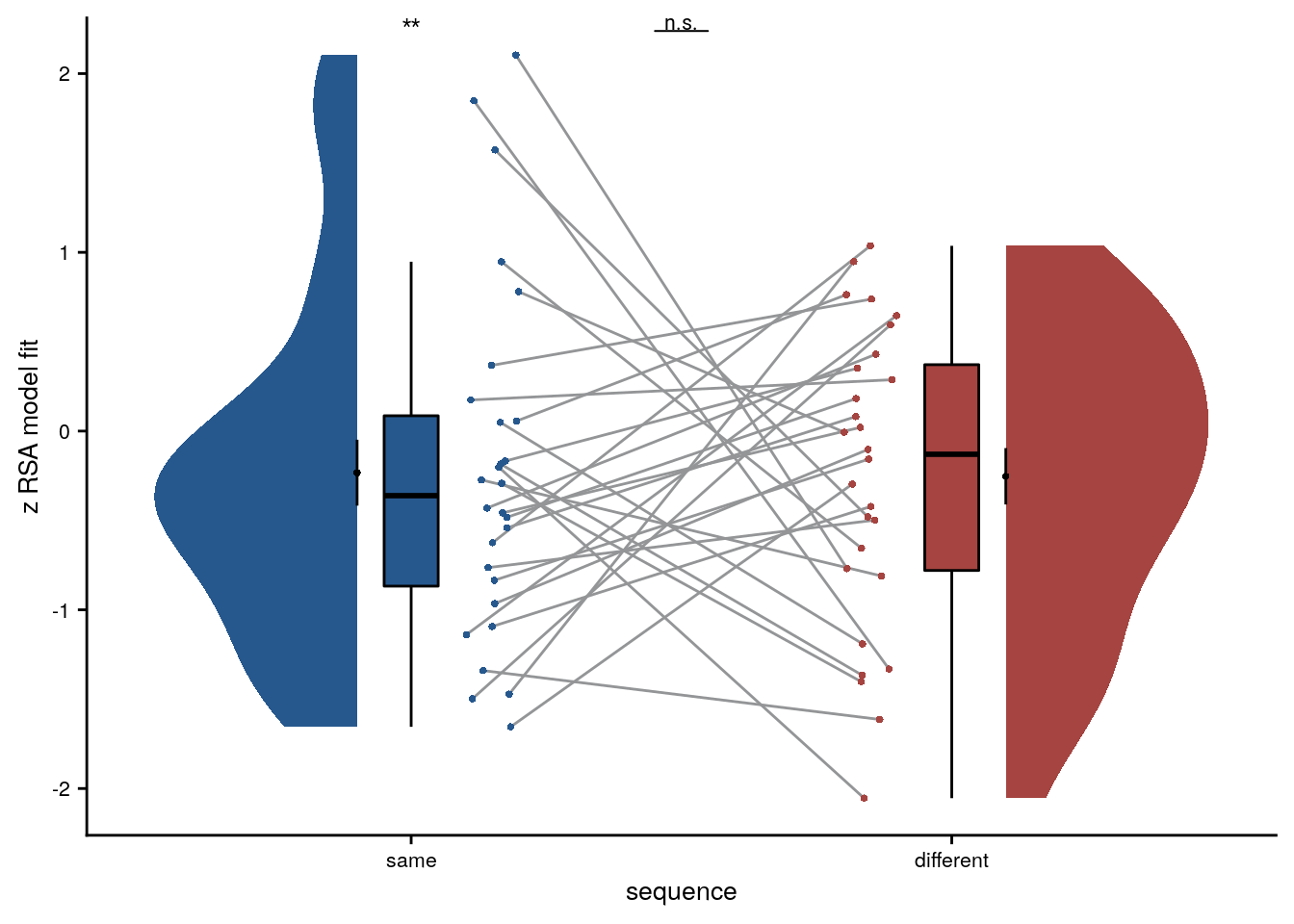
Mixed Effects
Test the interaction between sequence membership and virtual time on alEC representational change in mixed model analysis.
# get the data
rsa_dat_alEC <- rsa_dat %>% filter(roi == "alEC_lr")
# test the interaction for alEC
# maximal random effect structure --> singular fit
formula <- "ps_change ~ vir_time_diff * same_day_dv + (1 + vir_time_diff * same_day_dv | sub_id)"
lmm_full = lme4::lmer(formula, data=rsa_dat_alEC, REML=FALSE)## boundary (singular) fit: see ?isSingular# no correlations with random intercept --> singular fit
formula <- "ps_change ~ vir_time_diff * same_day_dv + (1 + vir_time_diff * same_day_dv || sub_id)"
lmm_full = lme4::lmer(formula, data=rsa_dat_alEC, REML=FALSE)## boundary (singular) fit: see ?isSingular# random intercepts and random slopes only for the critical interaction --> singular fit
formula <- "ps_change ~ vir_time_diff * same_day_dv + (1 + vir_time_diff : same_day_dv || sub_id)"
lmm_full = lme4::lmer(formula, data=rsa_dat_alEC, REML=FALSE)## boundary (singular) fit: see ?isSingular# random slopes for critical interactions
set.seed(378) # set seed for reproducibility
formula <- "ps_change ~ vir_time_diff * same_day_dv + (0 + vir_time_diff : same_day_dv | sub_id)"
lmm_full = lme4::lmer(formula, data=rsa_dat_alEC, REML=FALSE)## boundary (singular) fit: see ?isSingularsummary(lmm_full, corr = FALSE)## Linear mixed model fit by maximum likelihood ['lmerMod']
## Formula: ps_change ~ vir_time_diff * same_day_dv + (0 + vir_time_diff:same_day_dv | sub_id)
## Data: rsa_dat_alEC
##
## AIC BIC logLik deviance df.resid
## -29766.7 -29727.3 14889.4 -29778.7 5314
##
## Scaled residuals:
## Min 1Q Median 3Q Max
## -4.5825 -0.6461 0.0014 0.6380 4.1761
##
## Random effects:
## Groups Name Variance Std.Dev.
## sub_id vir_time_diff:same_day_dv 0.000000 0.00000
## Residual 0.000217 0.01473
## Number of obs: 5320, groups: sub_id, 28
##
## Fixed effects:
## Estimate Std. Error t value
## (Intercept) 0.0002612 0.0002521 1.036
## vir_time_diff -0.0005716 0.0002549 -2.242
## same_day_dv 0.0001285 0.0002521 0.510
## vir_time_diff:same_day_dv -0.0002320 0.0002549 -0.910
## convergence code: 0
## boundary (singular) fit: see ?isSingular# tidy summary of the fixed effects that calculates 95% CIs
lmm_full_bm <- broom.mixed::tidy(lmm_full, effects = "fixed", conf.int=TRUE, conf.method="profile")## Computing profile confidence intervals ...# tidy summary of the random effects
lmm_full_bm_re <- broom.mixed::tidy(lmm_full, effects = "ran_pars")
# test against reduced model
set.seed(370) # set seed for reproducibility
lmm_reduced <- update(lmm_full, ~ . - vir_time_diff:same_day_dv)## boundary (singular) fit: see ?isSingularlmm_aov <- anova(lmm_reduced, lmm_full)Mixed Model: Fixed effect of interaction of virtual time with sequence identity on alEC pattern similarity change \(\chi^2\)(1)=0.83, p=0.363
alEC: virtual time for all event pairs
Because there is no significant difference when we look at event pairs from the same vs. different days in the above analysis, we collapse across all comparisons to test for an effect of virtual time on entorhinal pattern similarity change.
Summary Statistics
set.seed(110) # set seed for reproducibility
# do RSA using linear model and calculate z-score for model fit from 1000 permutations
rsa_fit_ec <- rsa_dat %>%
filter(roi == "alEC_lr") %>%
group_by(sub_id) %>%
# run the linear model
do(z = lm_perm_jb(in_dat = ., lm_formula = "ps_change ~ vir_time_diff", nsim = n_perm)) %>%
mutate(z = list(setNames(z, c("z_intercept", "z_virtual_time")))) %>%
unnest_wider(z)
# run a group-level t-test on the RSA fits from the first level in alEC for both within-day and across days
stats <- rsa_fit_ec %>%
select(z_virtual_time) %>%
paired_t_perm_jb (., n_perm = n_perm)
# Cohen's d with Hedges' correction for one sample using non-central t-distribution for CI
d<-cohen.d(d=rsa_fit_ec$z_virtual_time,
f=NA, paired=TRUE, hedges.correction=TRUE, noncentral=TRUE)
stats$d <- d$estimate
stats$dCI_low <- d$conf.int[[1]]
stats$dCI_high <- d$conf.int[[2]]
# print results
huxtable(stats) %>% theme_article()| estimate | statistic | p.value | p_perm | parameter | conf.low | conf.high | method | alternative | d | dCI_low | dCI_high |
|---|---|---|---|---|---|---|---|---|---|---|---|
| -0.335 | -2.31 | 0.029 | 0.0294 | 27 | -0.634 | -0.0371 | One Sample t-test | two.sided | -0.423 | -0.835 | -0.0451 |
Summary Statistics: t-test against 0 for virtual time for all pairs in alEC
t27=-2.31, p=0.029, d=-0.42, 95% CI [-0.84, -0.05]
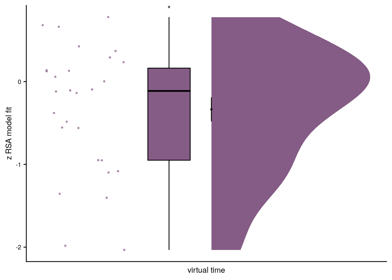
Linear Mixed Effects
When fitting a linear mixed effects model to test the effect of virtual time on pattern similarity change in the alEC, we thus use all pairwise comparisons. Due to singular fits we reduce the random effects structure to only include random slopes for virtual time. The model is still singular, but we keep these random slopes in the model to avoid anti-conservativity and to account for the within-subject dependencies.
# extract the comparisons from the same day
rsa_dat_ec <- rsa_dat %>% filter(roi == "alEC_lr")
# define the full model with virtual time difference as
# fixed effect and random intercepts for subject --> singular fit
formula <- "ps_change ~ vir_time_diff + (1 + vir_time_diff | sub_id)"
lmm_full <- lme4::lmer(formula, data = rsa_dat_ec, REML = FALSE)## boundary (singular) fit: see ?isSingular# remove the correlation between random slopes and intercepts --> still singular
formula <- "ps_change ~ vir_time_diff + (1 + vir_time_diff || sub_id)"
lmm_full <- lme4::lmer(formula, data = rsa_dat_ec, REML = FALSE)## boundary (singular) fit: see ?isSingular# keep only random slopes --> still singular
set.seed(301) # set seed for reproducibility
formula <- "ps_change ~ vir_time_diff + (0 + vir_time_diff | sub_id)"
lmm_full <- lme4::lmer(formula, data = rsa_dat_ec, REML = FALSE)## boundary (singular) fit: see ?isSingular#lmm_full = lme4::lmer(formula, data=rsa_dat_mtl, REML=FALSE,
# control = lmerControl(optimizer ="bobyqa", optCtrl=list(maxfun=100000)))
#lmm_full = lmer(formula, data=rsa_dat_mtl, REML=FALSE,
# control = lmerControl(optimizer ='nloptwrap',
# optCtrl=list(method='NLOPT_LN_NELDERMEAD', maxfun=100000)))
#lmm_full = lme4::lmer(formula, data=rsa_dat_mtl, REML=FALSE,
# control = lmerControl(optimizer ='optimx', optCtrl=list(method='nlminb')))
summary(lmm_full, corr=FALSE)## Linear mixed model fit by maximum likelihood ['lmerMod']
## Formula: ps_change ~ vir_time_diff + (0 + vir_time_diff | sub_id)
## Data: rsa_dat_ec
##
## AIC BIC logLik deviance df.resid
## -29769.8 -29743.5 14888.9 -29777.8 5316
##
## Scaled residuals:
## Min 1Q Median 3Q Max
## -4.5888 -0.6468 0.0016 0.6373 4.1684
##
## Random effects:
## Groups Name Variance Std.Dev.
## sub_id vir_time_diff 0.0000000 0.00000
## Residual 0.0002171 0.01473
## Number of obs: 5320, groups: sub_id, 28
##
## Fixed effects:
## Estimate Std. Error t value
## (Intercept) 0.0001670 0.0002020 0.827
## vir_time_diff -0.0004237 0.0002023 -2.095
## convergence code: 0
## boundary (singular) fit: see ?isSingular# tidy summary of the fixed effects that calculates 95% CIs
lmm_full_bm <- broom.mixed::tidy(lmm_full, effects = "fixed", conf.int=TRUE, conf.method="profile")## Computing profile confidence intervals ...# tidy summary of the random effects
lmm_full_bm_re <- broom.mixed::tidy(lmm_full, effects = "ran_pars")
# test against reduced model
set.seed(317) # set seed for reproducibility
formula <- "ps_change ~ 1 + (0 + vir_time_diff | sub_id)"
lmm_no_vir_time <- lme4::lmer(formula, data = rsa_dat_ec, REML = FALSE)## boundary (singular) fit: see ?isSingularlmm_aov <- anova(lmm_no_vir_time, lmm_full)Mixed Model: Fixed effect of virtual time on alEC pattern similarity change (all pairs) \(\chi^2\)(1)=4.39, p=0.036
Make mixed model summary table that includes overview of fixed and random effects as well as the model comparison to the nested (reduced) model.
fe_names <- c("intercept", "virtual time")
re_groups <- c(rep("participant",1), "residual")
re_names <- c("virtual time (SD)", "SD")
lmm_hux <- make_lme_huxtable(fix_df=lmm_full_bm,
ran_df = lmm_full_bm_re,
aov_mdl = lmm_aov,
fe_terms =fe_names,
re_terms = re_names,
re_groups = re_groups,
lme_form = gsub(" ", "", paste0(deparse(formula(lmm_full)),
collapse = "", sep="")),
caption = "Mixed Model: Virtual time explains representational change in the anterior-lateral entorhinal cortex (all events)")
# convert the huxtable to a flextable for word export
stable_lme_alEC_virtime_all_events <- convert_huxtable_to_flextable(ht = lmm_hux)
# print to screen
theme_article(lmm_hux)| fixed effects | ||||||
|---|---|---|---|---|---|---|
| term | estimate | SE | t-value | 95% CI | ||
| intercept | 0.000167 | 0.000202 | 0.83 | -0.000229 | 0.000563 | |
| virtual time | -0.000424 | 0.000202 | -2.09 | -0.000820 | -0.000027 | |
| random effects | ||||||
| group | term | estimate | ||||
| participant | virtual time (SD) | 0.000000 | ||||
| residual | SD | 0.014734 | ||||
| model comparison | ||||||
| model | npar | AIC | LL | X2 | df | p |
| reduced model | 3 | -29767.39 | 14886.69 | |||
| full model | 4 | -29769.77 | 14888.89 | 4.39 | 1 | 0.036 |
| model: ps_change~vir_time_diff+(0+vir_time_diff|sub_id); SE: standard error, CI: confidence interval, SD: standard deviation, npar: number of parameters, LL: log likelihood, df: degrees of freedom, corr.: correlation | ||||||
Visualize the effects.
lmm_full_bm <- lmm_full_bm %>%
mutate(term=as.factor(term))
# dot plot of Fixed Effect Coefficients with CIs
sfigmm_k <- ggplot(data = lmm_full_bm[2,], aes(x = term, color = term)) +
geom_hline(yintercept = 0, colour="black", linetype="dotted") +
geom_errorbar(aes(ymin = conf.low, ymax = conf.high, width = NA), size = 0.5) +
geom_point(aes(y = estimate), shape = 16, size = 1) +
scale_fill_manual(values = unname(alEC_colors["main"])) +
scale_color_manual(values = unname(alEC_colors["main"]), labels = c("Virtual Time")) +
labs(x = "virtual time", y="fixed effect\ncoefficient", color = "Time Metric") +
guides(color = "none") +
annotate(geom = "text", x = 1, y = Inf, label = "*", hjust = 0.5, vjust = 1, size = 8/.pt, family=font2use) +
theme_cowplot() +
theme(plot.title = element_text(hjust = 0.5), axis.text.x=element_blank())
sfigmm_k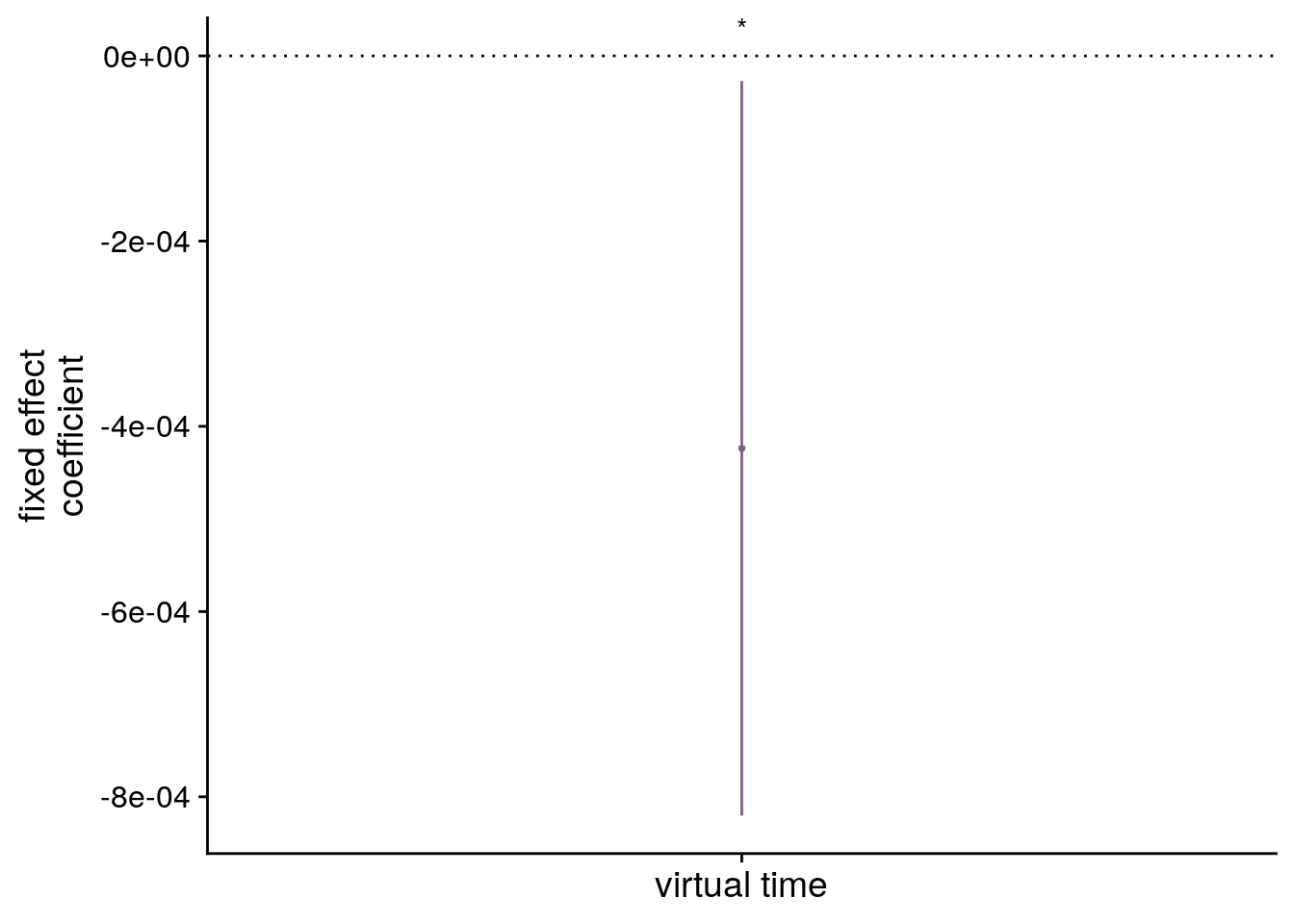
# estimate marginal means for each model term by omitting the terms argument
lmm_full_emm <- ggeffects::ggpredict(lmm_full, ci.lvl = 0.95) %>% get_complete_df()
# plot marginal means
sfigmm_l <- ggplot(data = lmm_full_emm, aes(color = group)) +
geom_line(aes(x, predicted)) +
geom_ribbon(aes(x, ymin = conf.low, ymax = conf.high, fill = group), alpha = .2, linetype=0) +
scale_color_manual(values = unname(alEC_colors["main"])) +
scale_fill_manual(values = unname(alEC_colors["main"])) +
ylab('estimated\nmarginal means') +
xlab('z virtual time') +
guides(color = "none", fill = "none") +
theme_cowplot()
sfigmm_l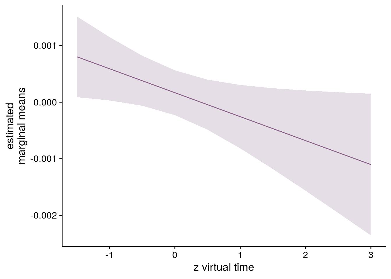
Pattern Similarity Change Visualization
To further visualize the effect, lets make a plot of the raw pattern similarity change for high vs. low temporal distances, averaged across all pairs.
# get data from alEC
rsa_dat_ec <- rsa_dat %>%
filter(roi == "alEC_lr")
# for each subject dichotomize virtual time difference
# based on a median split, then average high/low temporal distances
ps_change_means <-rsa_dat_ec %>% group_by(sub_id) %>%
mutate(temp_dist = sjmisc::dicho(vir_time_diff, as.num = TRUE)+1) %>%
group_by(sub_id, temp_dist) %>%
summarise(ps_change = mean(ps_change), .groups = 'drop')
# make the high/low temporal distance variable a factor
ps_change_means <- ps_change_means %>%
mutate(
temp_dist = as.numeric(temp_dist),
temp_dist_f = factor(temp_dist),
temp_dist_f = plyr::mapvalues(temp_dist, from = c(1,2), to = c("low", "high")),
temp_dist_f = factor(temp_dist_f, levels= c("low", "high")),
roi = "alEC")
# add a column with subject-specific jitter
# generate custom repeating jitter (multiply with -1/1 to shift towards each other)
ps_change_means <- ps_change_means %>%
mutate(
x_jit = as.numeric(temp_dist) + rep(jitter(rep(0,n_subs), amount = 0.05), each=2) * rep(c(-1,1),n_subs))
f6c<- ggplot(data=ps_change_means, aes(x=temp_dist, y=ps_change, fill = roi, color = roi)) +
gghalves::geom_half_violin(data = ps_change_means %>% filter(temp_dist_f == "low"),
aes(x=temp_dist, y=ps_change),
position=position_nudge(-0.1),
side = "l", color = NA) +
gghalves::geom_half_violin(data = ps_change_means %>% filter(temp_dist_f == "high"),
aes(x=temp_dist, y=ps_change),
position=position_nudge(0.1),
side = "r", color = NA) +
geom_boxplot(aes(group = temp_dist),width = .1, colour = "black", outlier.shape = NA) +
geom_line(aes(x = x_jit, group=sub_id,), color = ultimate_gray,
position = position_nudge(c(0.15, -0.15))) +
geom_point(aes(x=x_jit), position = position_nudge(c(0.15, -0.15)),
shape=16, size = 1) +
stat_summary(fun = mean, geom = "point", size = 1, shape = 16,
position = position_nudge(c(-0.1, 0.1)), colour = "black") +
stat_summary(fun.data = mean_se, geom = "errorbar",
position = position_nudge(c(-0.1, 0.1)), colour = "black", width = 0, size = 0.5) +
scale_fill_manual(values = unname(alEC_colors["main"])) +
scale_color_manual(values = unname(alEC_colors["main"]))+
scale_x_continuous(breaks = c(1,2), labels=c("low", "high")) +
ylab('pattern similarity change') + xlab('temporal distance') +
guides(fill = "none", color = "none") +
theme_cowplot() +
theme(text = element_text(size=10), axis.text = element_text(size=8),
legend.position = "none", strip.background = element_blank(), strip.text = element_blank())
f6c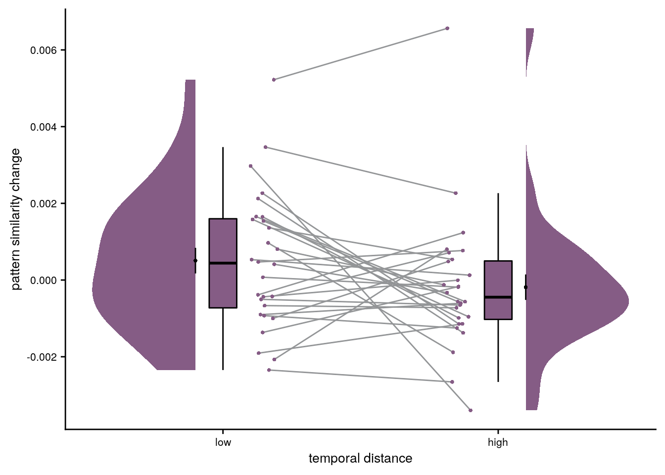
# save source data
source_dat <-ggplot_build(f6c)$data[[4]]
readr::write_tsv(source_dat %>% select(x, y, group),
file = file.path(dirs$source_dat_dir, "f6c.txt"))Now we are ready to make figure 6 of the manuscript.
layoutBC <- "BCC"
f6bc <- f6b + f6c +
plot_layout(design = layoutBC)
f6a_guide <- guide_area() + f6a +
plot_layout(design = "ABBBB", guides = "collect")
layout <- "
AAA
BCC
BCC
BCC"
f6 <- f6a + f6b + f6c +
plot_layout(design = layout) &
theme(text = element_text(size=10, family = font2use),
axis.text = element_text(size=8),
legend.position = 'none') &
plot_annotation(theme = theme(plot.margin = margin(t=0, r=-5, b=0, l=-5, unit="pt")),
tag_levels = 'A')
f6[[1]] <- f6[[1]] + theme_no_ticks()
# save and print
fn <- here("figures", "f6")
ggsave(paste0(fn, ".pdf"), plot=f6, units = "cm",
width = 8.8, height = 12, dpi = "retina", device = cairo_pdf)
ggsave(paste0(fn, ".png"), plot=f6, units = "cm",
width = 8.8, height = 12, dpi = "retina", device = "png")
Figure 6. The anterior-lateral entorhinal cortex uses a shared representational format for relations of events from the same and different sequences. A. The anterior-lateral entorhinal cortex region of interest is displayed on the MNI template with voxels outside the field of view shown in lighter shades of gray. Color code denotes probability of a voxel to be included based on participant-specific masks (see Methods). B. Z-values for participant-specific RSA model fits show a negative relationship between pattern similarity change and virtual temporal distances when collapsing across all event pairs. C. To illustrate the effect in B, raw pattern similarity change in the anterior-lateral entorhinal cortex was averaged for events separated by low and high temporal distances based on a median split. * p<0.05
alEC: virtual time for all event pairs when including order & real time
We also asked whether virtual time explains alEC pattern similarity change when including order and real time in the model as predictors of no interest. Based on the findings above, we collapse across event pairs from the same and from different sequences.
Summary Statistics
# SUMMARY STATS alEC WITH ORDER AND REAL TIME
set.seed(59) # set seed for reproducibility
# extract all comparisons from the same day
rsa_dat_alEC <- rsa_dat %>%
filter(roi == "alEC_lr")
# do RSA using linear model and calculate z-score for model fit from permutations
rsa_fit_alEC_mult_reg <- rsa_dat_alEC %>% group_by(sub_id) %>%
# run the linear model
do(z = lm_perm_jb(in_dat = .,
lm_formula = "ps_change ~ vir_time_diff + order_diff + real_time_diff",
nsim = n_perm)) %>%
mutate(z = list(setNames(z, c("z_intercept", "z_virtual_time", "z_order", "z_real_time")))) %>%
unnest_longer(z) %>%
filter(z_id != "z_intercept")
# run group-level t-tests on the RSA fits from the first level in alEC (virtual time)
stats <- rsa_fit_alEC_mult_reg %>%
filter(z_id =="z_virtual_time") %>%
select(z) %>%
paired_t_perm_jb (., n_perm = n_perm)
# Cohen's d with Hedges' correction for one sample using non-central t-distribution for CI
d<-cohen.d(d=(rsa_fit_alEC_mult_reg %>% filter(z_id == "z_virtual_time"))$z, f=NA, paired=TRUE, hedges.correction=TRUE, noncentral=TRUE)
stats$d <- d$estimate
stats$dCI_low <- d$conf.int[[1]]
stats$dCI_high <- d$conf.int[[2]]
# print results
huxtable(stats) %>% theme_article()| estimate | statistic | p.value | p_perm | parameter | conf.low | conf.high | method | alternative | d | dCI_low | dCI_high |
|---|---|---|---|---|---|---|---|---|---|---|---|
| -0.144 | -0.702 | 0.489 | 0.495 | 27 | -0.567 | 0.278 | One Sample t-test | two.sided | -0.129 | -0.513 | 0.245 |
t27=-0.7, p=0.495, d=-0.13, 95% CI [-0.51, 0.25]
# make z_id a factor and reorder it
rsa_fit_alEC_mult_reg <- rsa_fit_alEC_mult_reg %>% mutate(
z_id = factor(z_id, levels = c("z_virtual_time", "z_order", "z_real_time")))
# raincloud plot
sfig7_b <- ggplot(rsa_fit_alEC_mult_reg, aes(x=z_id, y=z, fill = z_id, colour = z_id)) +
gghalves::geom_half_violin(position=position_nudge(0.1),
side = "r", color = NA) +
geom_point(aes(x = as.numeric(z_id)-0.2), alpha = 0.7,
position = position_jitter(width = .1, height = 0),
shape=16, size = 1) +
geom_boxplot(position = position_nudge(x = 0, y = 0),
width = .1, colour = "black", outlier.shape = NA) +
stat_summary(fun = mean, geom = "point", size = 1, shape = 16,
position = position_nudge(.1), colour = "black") +
stat_summary(fun.data = mean_se, geom = "errorbar",
position = position_nudge(.1), colour = "black", width = 0, size = 0.5)+
ylab('z RSA model fit') + xlab('time metric') +
scale_x_discrete(labels = c("virtual time", "order", "real time")) +
scale_color_manual(values = c(unname(alEC_colors["main"]), time_colors[c(2,3)]), name = "time metric",
labels = c("virtual time", "order", "real time")) +
scale_fill_manual(values = c(unname(alEC_colors["main"]), time_colors[c(2,3)])) +
guides(fill = "none", color=guide_legend(override.aes=list(fill=NA, alpha = 1, size=2))) +
theme_cowplot() +
theme(text = element_text(size=10), axis.text = element_text(size=8),
legend.position = "none")
sfig7_b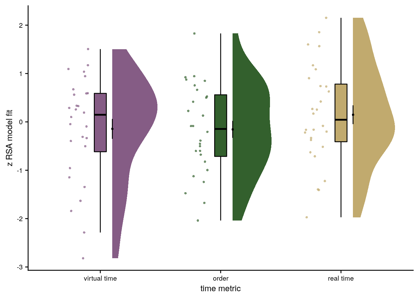
Try real time in alEC for response letter.
set.seed(110) # set seed for reproducibility
# do RSA using linear model and calculate z-score for model fit from 1000 permutations
rsa_fit_ec <- rsa_dat %>%
filter(roi == "alEC_lr") %>%
group_by(sub_id) %>%
# run the linear model
do(z = lm_perm_jb(in_dat = ., lm_formula = "ps_change ~ real_time_diff", nsim = n_perm)) %>%
mutate(z = list(setNames(z, c("z_intercept", "z_real_time")))) %>%
unnest_wider(z)
# run a group-level t-test on the RSA fits from the first level in alEC for both within-day and across days
stats <- rsa_fit_ec %>%
select(z_real_time) %>%
paired_t_perm_jb (., n_perm = n_perm)
# Cohen's d with Hedges' correction for one sample using non-central t-distribution for CI
d<-cohen.d(d=rsa_fit_ec$z_real_time,
f=NA, paired=TRUE, hedges.correction=TRUE, noncentral=TRUE)
stats$d <- d$estimate
stats$dCI_low <- d$conf.int[[1]]
stats$dCI_high <- d$conf.int[[2]]
# print results
huxtable(stats) %>% theme_article()| estimate | statistic | p.value | p_perm | parameter | conf.low | conf.high | method | alternative | d | dCI_low | dCI_high |
|---|---|---|---|---|---|---|---|---|---|---|---|
| -0.296 | -2.17 | 0.0389 | 0.0382 | 27 | -0.576 | -0.0162 | One Sample t-test | two.sided | -0.398 | -0.807 | -0.021 |
Summary Statistics: t-test against 0 for real time for all pairs in alEC
t27=-2.17, p=0.038, d=-0.40, 95% CI [-0.81, -0.02]
# run group-level t-tests on the RSA fits from the first level in alEC [real time]
stats <- rsa_fit_alEC_mult_reg %>%
filter(z_id =="z_real_time") %>%
select(z) %>%
paired_t_perm_jb (., n_perm = n_perm)
# Cohen's d with Hedges' correction for one sample using non-central t-distribution for CI
d<-cohen.d(d=(rsa_fit_alEC_mult_reg %>% filter(z_id == "z_virtual_time"))$z, f=NA, paired=TRUE, hedges.correction=TRUE, noncentral=TRUE)
stats$d <- d$estimate
stats$dCI_low <- d$conf.int[[1]]
stats$dCI_high <- d$conf.int[[2]]
huxtable(stats) %>% theme_article()| estimate | statistic | p.value | p_perm | parameter | conf.low | conf.high | method | alternative | d | dCI_low | dCI_high |
|---|---|---|---|---|---|---|---|---|---|---|---|
| 0.148 | 0.764 | 0.451 | 0.446 | 27 | -0.25 | 0.547 | One Sample t-test | two.sided | -0.129 | -0.513 | 0.245 |
t27=0.76, p=0.446, d=-0.13, 95% CI [-0.51, 0.25]
# run group-level t-tests on the RSA fits from the first level in alEC [order]
stats <- rsa_fit_alEC_mult_reg %>%
filter(z_id =="z_order") %>%
select(z) %>%
paired_t_perm_jb (., n_perm = n_perm)
# Cohen's d with Hedges' correction for one sample using non-central t-distribution for CI
d<-cohen.d(d=(rsa_fit_alEC_mult_reg %>% filter(z_id == "z_order"))$z, f=NA, paired=TRUE, hedges.correction=TRUE, noncentral=TRUE)
stats$d <- d$estimate
stats$dCI_low <- d$conf.int[[1]]
stats$dCI_high <- d$conf.int[[2]]
huxtable(stats) %>% theme_article()| estimate | statistic | p.value | p_perm | parameter | conf.low | conf.high | method | alternative | d | dCI_low | dCI_high |
|---|---|---|---|---|---|---|---|---|---|---|---|
| -0.155 | -0.885 | 0.384 | 0.384 | 27 | -0.514 | 0.204 | One Sample t-test | two.sided | -0.162 | -0.549 | 0.211 |
t27=-0.89, p=0.384, d=-0.16, 95% CI [-0.55, 0.21]
Linear Mixed Effects
# LME alEC WITH ORDER AND REAL TIME
set.seed(59) # set seed for reproducibility
# extract all comparisons from the same day
rsa_dat_alEC <- rsa_dat %>%
filter(roi == "alEC_lr")
# define the full model with virtual time difference, order difference and real time difference as
# fixed effects and random intercepts and random slopes for all effects
# fails to converge and is singular after restart
formula <- "ps_change ~ vir_time_diff + order_diff + real_time_diff + (1+vir_time_diff + order_diff + real_time_diff | sub_id)"
lmm_full <- lme4::lmer(formula, data = rsa_dat_alEC, REML = FALSE)## boundary (singular) fit: see ?isSingular# remove the correlation between random slopes and random intercepts
formula <- "ps_change ~ vir_time_diff + order_diff + real_time_diff + (1+vir_time_diff + order_diff + real_time_diff || sub_id)"
lmm_full <- lme4::lmer(formula, data = rsa_dat_alEC, REML = FALSE)## boundary (singular) fit: see ?isSingular# thus we reduce the random effect structure by excluding random slopes for the fixed effects of no interest
# as above this results in a singular fit (the random intercept variance estimated to be 0)
formula <- "ps_change ~ vir_time_diff + order_diff + real_time_diff + (1+vir_time_diff | sub_id)"
lmm_full <- lme4::lmer(formula, data = rsa_dat_alEC, REML = FALSE)## boundary (singular) fit: see ?isSingular# next step is to remove the correlation between random slopes and random intercepts
formula <- "ps_change ~ vir_time_diff + order_diff + real_time_diff + (1+vir_time_diff || sub_id)"
lmm_full <- lme4::lmer(formula, data = rsa_dat_alEC, REML = FALSE)## boundary (singular) fit: see ?isSingular# we thus reduce further and keep only the random slopes for virtual time differences, but fit is still singular
set.seed(332) # set seed for reproducibility
formula <- "ps_change ~ vir_time_diff + order_diff + real_time_diff + (0 + vir_time_diff | sub_id)"
lmm_full <- lme4::lmer(formula, data = rsa_dat_alEC, REML = FALSE)## boundary (singular) fit: see ?isSingularsummary(lmm_full, corr = FALSE)## Linear mixed model fit by maximum likelihood ['lmerMod']
## Formula: ps_change ~ vir_time_diff + order_diff + real_time_diff + (0 + vir_time_diff | sub_id)
## Data: rsa_dat_alEC
##
## AIC BIC logLik deviance df.resid
## -29766.6 -29727.1 14889.3 -29778.6 5314
##
## Scaled residuals:
## Min 1Q Median 3Q Max
## -4.5966 -0.6483 0.0047 0.6405 4.1872
##
## Random effects:
## Groups Name Variance Std.Dev.
## sub_id vir_time_diff 0.0000000 0.00000
## Residual 0.0002171 0.01473
## Number of obs: 5320, groups: sub_id, 28
##
## Fixed effects:
## Estimate Std. Error t value
## (Intercept) 0.0001670 0.0002020 0.827
## vir_time_diff -0.0005762 0.0005307 -1.086
## order_diff -0.0007122 0.0008621 -0.826
## real_time_diff 0.0008616 0.0009656 0.892
## convergence code: 0
## boundary (singular) fit: see ?isSingular# tidy summary of the fixed effects that calculates 95% CIs
lmm_full_bm <- broom.mixed::tidy(lmm_full, effects = "fixed", conf.int=TRUE, conf.method="profile")## Computing profile confidence intervals ...# tidy summary of the random effects
lmm_full_bm_re <- broom.mixed::tidy(lmm_full, effects = "ran_pars")
# one way of testing for significance is by comparing the likelihood against a simpler model.
# Here, we drop the effect of virtual time difference and run an ANOVA. See e.g. Bodo Winter tutorial
set.seed(321) # set seed for reproducibility
formula <- "ps_change ~ order_diff + real_time_diff + (0 + vir_time_diff | sub_id)"
lmm_no_vir_time <- lme4::lmer(formula, data = rsa_dat_alEC, REML = FALSE)## boundary (singular) fit: see ?isSingularlmm_aov <- anova(lmm_no_vir_time, lmm_full)
lmm_aov| npar | AIC | BIC | logLik | deviance | Chisq | Df | Pr(>Chisq) |
|---|---|---|---|---|---|---|---|
| 5 | -2.98e+04 | -2.97e+04 | 1.49e+04 | -2.98e+04 | |||
| 6 | -2.98e+04 | -2.97e+04 | 1.49e+04 | -2.98e+04 | 1.18 | 1 | 0.278 |
Mixed Model: Fixed effect of virtual time on alEC (all event pairs) pattern similarity change with order and real time in model \(\chi^2\)(1)=1.18, p=0.278
Make mixed model summary table that includes overview of fixed and random effects as well as the model comparison to the nested (reduced) model.
fe_names <- c("intercept", "virtual time", "order", "real time")
re_groups <- c(rep("participant",1), "residual")
re_names <- c("virtual time (SD)", "SD")
lmm_hux <- make_lme_huxtable(fix_df=lmm_full_bm,
ran_df = lmm_full_bm_re,
aov_mdl = lmm_aov,
fe_terms =fe_names,
re_terms = re_names,
re_groups = re_groups,
lme_form = gsub(" ", "", paste0(deparse(formula(lmm_full)),
collapse = "", sep="")),
caption = "Mixed Model: Virtual time does not explain representational change for different-sequence events in the anterior-lateral entorhinal cortex when including order and real time in the model")
# convert the huxtable to a flextable for word export
stable_lme_alEC_virtime_all_comps_time_metrics <- convert_huxtable_to_flextable(ht = lmm_hux)
# print to screen
theme_article(lmm_hux)| fixed effects | ||||||
|---|---|---|---|---|---|---|
| term | estimate | SE | t-value | 95% CI | ||
| intercept | 0.000167 | 0.000202 | 0.83 | -0.000229 | 0.000563 | |
| virtual time | -0.000576 | 0.000531 | -1.09 | -0.001617 | 0.000464 | |
| order | -0.000712 | 0.000862 | -0.83 | -0.002402 | 0.000978 | |
| real time | 0.000862 | 0.000966 | 0.89 | -0.001031 | 0.002754 | |
| random effects | ||||||
| group | term | estimate | ||||
| participant | virtual time (SD) | 0.000000 | ||||
| residual | SD | 0.014733 | ||||
| model comparison | ||||||
| model | npar | AIC | LL | X2 | df | p |
| reduced model | 5 | -29767.41 | 14888.71 | |||
| full model | 6 | -29766.59 | 14889.30 | 1.18 | 1 | 0.278 |
| model: ps_change~vir_time_diff+order_diff+real_time_diff+(0+vir_time_diff|sub_id); SE: standard error, CI: confidence interval, SD: standard deviation, npar: number of parameters, LL: log likelihood, df: degrees of freedom, corr.: correlation | ||||||
Mixed model plots.
# set RNG
set.seed(23)
lmm_full_bm <- lmm_full_bm %>%
mutate(term=as.factor(term) %>%
factor(levels = c("vir_time_diff", "order_diff", "real_time_diff")))
# dot plot of Fixed Effect Coefficients with CIs
sfig7_c <- ggplot(data = lmm_full_bm[2:4,], aes(x = term, color = term)) +
geom_hline(yintercept = 0, colour="black", linetype="dotted") +
geom_errorbar(aes(ymin = conf.low, ymax = conf.high, width = NA), size = 0.5) +
geom_point(aes(y = estimate), shape = 16, size = 1) +
scale_fill_manual(values = c(unname(alEC_colors["main"]), time_colors[c(2,3)])) +
scale_color_manual(values = c(unname(alEC_colors["main"]), time_colors[c(2,3)]), labels = c("Virtual Time", "Order", "Real Time")) +
labs(x = "time metric", y = "fixed effect\nestimate", color = "Time Metric") +
guides(color = "none", fill = "none") +
theme_cowplot() +
theme(plot.title = element_text(hjust = 0.5), axis.text.x=element_blank())
sfig7_c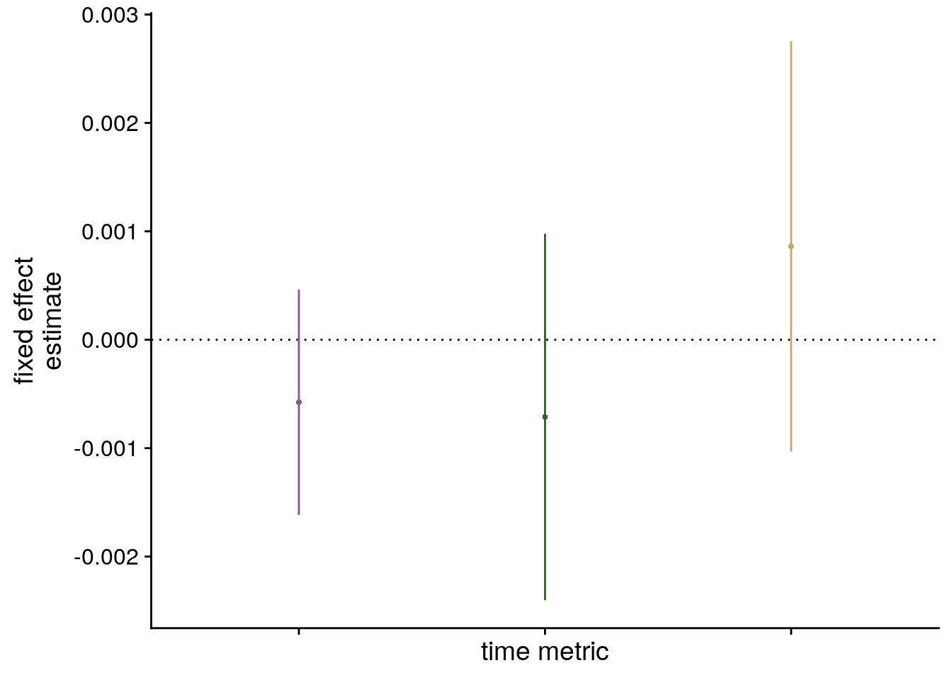
# estimate marginal means for each model term by omitting the terms argument
lmm_full_emm <- ggeffects::ggpredict(lmm_full, ci.lvl = 0.95) %>% get_complete_df
# convert the group variable to a factor to control the order of facets below
lmm_full_emm$group <- factor(lmm_full_emm$group, levels = c("vir_time_diff", "order_diff", "real_time_diff"))
# plot marginal means
sfig7_d <- ggplot(data = lmm_full_emm, aes(color = group)) +
geom_line(aes(x, predicted)) +
geom_ribbon(aes(x, ymin = conf.low, ymax = conf.high, fill = group), alpha = .2, linetype=0) +
scale_color_manual(values = c(unname(alEC_colors["main"]), time_colors[c(2,3)]), name = element_blank(),
labels = c("virtual time", "order", "real time")) +
scale_fill_manual(values = c(unname(alEC_colors["main"]), time_colors[c(2,3)])) +
ylab('estimated\nmarginal means') +
xlab('z time metric') +
guides(fill = "none", color= "none") +
theme_cowplot() +
theme(plot.title = element_text(hjust = 0.5), strip.background = element_blank(),
strip.text.x = element_blank())
sfig7_d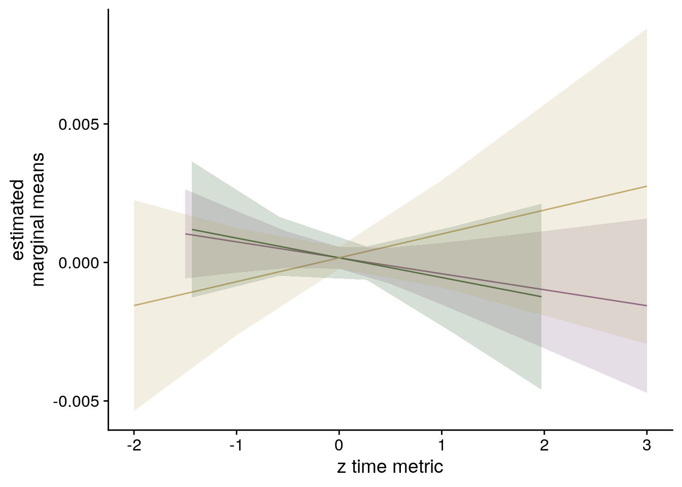
8.9.0.1 alEC Supplemental Figure
layout = "
AAABBBC
AAABBBD"
sfig7 <- sfig7_a + sfig7_b + sfig7_c + sfig7_d +
plot_layout(design = layout, guides = 'collect') &
theme(text = element_text(size=10, family = font2use),
axis.text = element_text(size=8),
legend.position = "bottom") &
plot_annotation(tag_levels = 'A')
# save and print to screen
fn <- here("figures", "sf07")
ggsave(paste0(fn, ".pdf"), plot=sfig7, units = "cm",
width = 17.4, height = 10, dpi = "retina", device = cairo_pdf)
ggsave(paste0(fn, ".png"), plot=sfig7, units = "cm",
width = 17.4, height = 10, dpi = "retina", device = "png")
Supplemental Figure 7. Pattern similarity change in the anterior-lateral entorhinal cortex. A. Relationship of pattern similarity change and temporal distances between events from the same and different sequences in the anterior-lateral entorhinal cortex. There was no statistically significant difference between correlations of virtual temporal distances and representational change in the anterior-lateral entorhinal cortex depending on whether event pairs were from the same or different sequences. Entorhinal representational change was negatively related to temporal distances between events from the same sequence (summary statistics: t24=-3.54, p=0.002, d=-0.69, 95% CI [-1.17, -0.27]; α=0.025, corrected for separate tests of events of the same and different sequences; three outliers excluded based on the boxplot criterion). The relationship between entorhinal pattern similarity change for events from different sequences was not statistically different from zero (summary statistics: t27=-1.60, p=0.122, d=-0.29, 95% CI [-0.69, 0.08]; α=0.025, corrected for separate tests of events of the same and different sequences). ** p<0.01 after outlier exclusion. B. Z-values show the relationship of the different time metrics to representational change in the anterior-lateral entorhinal cortex based on participant-specific multiple regression analyses. Analysis includes all pairs of events. C, D. Parameter estimates with 95% CI (C) and estimated marginal means (D) show the fixed effects of the three time metrics from the corresponding mixed model. A,B. Circles show participant-specific Z-values from summary statistics approach; boxplot shows median and upper/lower quartile along with whiskers extending to most extreme data point within 1.5 interquartile ranges above/below the upper/lower quartile; black circle with error bars corresponds to mean±S.E.M.; distribution shows probability density function of data points.
8.10 aHPC vs. alEC
The findings above suggest differences between how sequence memories in aHPC and alEC are shaped by virtual time depending on whether events from the same or from different sequences are compared. Let’s qualify these differences by running models with both ROIs.
Summary Statistics
Permutation-based repeated measures ANOVAs were carried out using the permuco package111 and we report generalized η2 as effect sizes computed using the afex-package112.
In the summary statistics approach, this comes down to a 2x2 repeated measures ANOVA with the factors ROI (aHPC vs. alEC) and sequence (same vs. different). We use a permutation-based repeated measures ANOVA to show there is a significant interaction between the two factors.
# sanity check & effect size: parametric ANOVA using
# run a 2x2 repeated measures ANOVA from afex package
aov_fit <- afex::aov_ez(id = "sub_id",
dv = "z_virtual_time",
data = rsa_fit,
within = c("roi", "same_day"), print.formula = TRUE, es="ges")## Formula send to aov_car: z_virtual_time ~ 1 + Error(sub_id/(roi * same_day))# print stats
aov_fit## Anova Table (Type 3 tests)
##
## Response: z_virtual_time
## Effect df MSE F ges p.value
## 1 roi 1, 27 0.82 3.10 + .024 .089
## 2 same_day 1, 27 1.22 7.41 * .082 .011
## 3 roi:same_day 1, 27 1.09 7.76 ** .076 .010
## ---
## Signif. codes: 0 '***' 0.001 '**' 0.01 '*' 0.05 '+' 0.1 ' ' 1set.seed(111) # set seed for reproducibility
# permutation repeated measures from permuco package (use factorial same_day variable)
aov_fit_perm <- permuco::aovperm(formula = z_virtual_time ~ roi * same_day_char + Error(sub_id/(roi*same_day_char)),
data = rsa_fit, method = "Rd_kheradPajouh_renaud", np =n_perm)
summary(aov_fit_perm)| SSn | dfn | SSd | dfd | MSEn | MSEd | F | parametric P(>F) | permutation P(>F) |
|---|---|---|---|---|---|---|---|---|
| 2.55 | 1 | 22.2 | 27 | 2.55 | 0.822 | 3.1 | 0.0895 | 0.0859 |
| 9.06 | 1 | 33 | 27 | 9.06 | 1.22 | 7.41 | 0.0112 | 0.0115 |
| 8.43 | 1 | 29.3 | 27 | 8.43 | 1.09 | 7.76 | 0.00964 | 0.0102 |
Summary Statistics: permutation-based repeated measures ANOVA (Rd_kheradPajouh_renaud method)
main effect of ROI: F1,27=3.1, p=0.086, \(\eta^2\)=0.02
main effect of sequence: F1,27=7.41, p=0.012, \(\eta^2\)=0.08
interaction ROI and sequence: F1,27=7.76, p=0.010, \(\eta^2\)=0.08
### Linear Mixed Effects {-}
To test whether the hippocampus and entorhinal cortex differentially represent virtual time between events within a virtual day and also virtual days, we also run a linear mixed model on pattern similarity change in both regions that includes event pairs that are from the same day, but also from different days. We include the fixed effects ROI (aHPC and alEC), day (same or different) and virtual time difference as well as their interaction in the model.
# get data from aHPC and alEC for within and across day comparisons
rsa_dat_mtl <- rsa_dat %>% filter(roi == "aHPC_lr" | roi == "alEC_lr")
# recode the ROI factor to -1 and 1
rsa_dat_mtl <- rsa_dat_mtl %>%
mutate(
roi_dv = plyr::mapvalues(roi, from = c("alEC_lr", "aHPC_lr"), to = c(-1, 1)))
# run LME for effect of time with factors same/different day vs. ROI
# random intercepts and all random slopes and interactions --> singular fit
formula <- "ps_change ~ vir_time_diff * same_day_dv * roi_dv + (1 + vir_time_diff * same_day_dv * roi_dv | sub_id)"
lmm_full = lme4::lmer(formula, data=rsa_dat_mtl, REML=FALSE,
control = lmerControl(optimizer ="bobyqa", optCtrl=list(maxfun=40000)))## boundary (singular) fit: see ?isSingular# remove correlation between random slopes and random intercepts --> singular fit
formula <- "ps_change ~ vir_time_diff * same_day_dv * roi_dv + (1 + vir_time_diff * same_day_dv * roi_dv || sub_id)"
lmm_full = lme4::lmer(formula, data=rsa_dat_mtl, REML=FALSE,
control = lmerControl(optimizer ="bobyqa", optCtrl=list(maxfun=40000)))## boundary (singular) fit: see ?isSingular# keep only highest-order interaction as random slopes
formula <- "ps_change ~ vir_time_diff * same_day_dv * roi_dv + (1 + vir_time_diff : same_day_dv : roi_dv | sub_id)"
lmm_full = lme4::lmer(formula, data=rsa_dat_mtl, REML=FALSE,
control = lmerControl(optimizer ="bobyqa", optCtrl=list(maxfun=40000)))## boundary (singular) fit: see ?isSingular#lmm_full = lme4::lmer(formula, data=rsa_dat_mtl, REML=FALSE,
# control = lmerControl(optimizer ='optimx', optCtrl=list(method='nlminb', maxit=100000)))
set.seed(398) # set seed for reproducibility
lmm_full = lme4::lmer(formula, data=rsa_dat_mtl, REML=FALSE,
control = lmerControl(optimizer ='nloptwrap',
optCtrl=list(method='NLOPT_LN_NELDERMEAD', maxfun=100000)))## boundary (singular) fit: see ?isSingularsummary(lmm_full, corr = FALSE)## Linear mixed model fit by maximum likelihood ['lmerMod']
## Formula: ps_change ~ vir_time_diff * same_day_dv * roi_dv + (1 + vir_time_diff:same_day_dv:roi_dv | sub_id)
## Data: rsa_dat_mtl
## Control: lmerControl(optimizer = "nloptwrap", optCtrl = list(method = "NLOPT_LN_NELDERMEAD", maxfun = 1e+05))
##
## AIC BIC logLik deviance df.resid
## -64704.2 -64595.1 32367.1 -64734.2 10625
##
## Scaled residuals:
## Min 1Q Median 3Q Max
## -5.9391 -0.5647 0.0096 0.5629 5.3781
##
## Random effects:
## Groups Name Variance Std.Dev. Corr
## sub_id (Intercept) 2.460e-07 0.0004960
## vir_time_diff:same_day_dv:roi_dv1 2.897e-08 0.0001702 -1.00
## vir_time_diff:same_day_dv:roi_dv-1 1.772e-07 0.0004209 -0.15 0.15
## Residual 1.332e-04 0.0115397
## Number of obs: 10640, groups: sub_id, 28
##
## Fixed effects:
## Estimate Std. Error t value
## (Intercept) -0.0001934 0.0002186 -0.885
## vir_time_diff 0.0002384 0.0001997 1.194
## same_day_dv -0.0001327 0.0001974 -0.672
## roi_dv-1 0.0004546 0.0002792 1.628
## vir_time_diff:same_day_dv 0.0005129 0.0002022 2.536
## vir_time_diff:roi_dv-1 -0.0008100 0.0002824 -2.868
## same_day_dv:roi_dv-1 0.0002612 0.0002792 0.936
## vir_time_diff:same_day_dv:roi_dv-1 -0.0007449 0.0002938 -2.535
## convergence code: 0
## boundary (singular) fit: see ?isSingular# tidy summary of the fixed effects that calculates 95% CIs
lmm_full_bm <- broom.mixed::tidy(lmm_full, effects = "fixed",
conf.int=TRUE, optimizer = 'bobyqa')
# tidy summary of the random effects
lmm_full_bm_re <- broom.mixed::tidy(lmm_full, effects = "ran_pars")
# compare to reduced model without interaction term
set.seed(351) # set seed for reproducibility
lmm_reduced <-update(lmm_full, ~ . - vir_time_diff:same_day_dv:roi_dv)## boundary (singular) fit: see ?isSingularlmm_aov <- anova(lmm_reduced, lmm_full)
lmm_aov| npar | AIC | BIC | logLik | deviance | Chisq | Df | Pr(>Chisq) |
|---|---|---|---|---|---|---|---|
| 14 | -6.47e+04 | -6.46e+04 | 3.24e+04 | -6.47e+04 | |||
| 15 | -6.47e+04 | -6.46e+04 | 3.24e+04 | -6.47e+04 | 6.31 | 1 | 0.012 |
Mixed Model: Fixed effect of interaction virtual time with sequence identity and ROI on pattern similarity change \(\chi^2\)(1)=6.31, p=0.012
Make mixed model summary table that includes overview of fixed and random effects as well as the model comparison to the nested (reduced) model.
fe_names <- c("intercept", "virtual time", "day", "ROI", "virtual time * day",
              "virtual time * ROI", "day * ROI", "virtual time * day * ROI")
re_groups <- c(rep("participant",6), "residual")
re_names <- c("intercept (SD)", "corr. intercept, virtual time:day:ROI1",
              "corr. intercept, virtual time:day:ROI-1", "virtual time:day:ROI1 (SD)",
              "corr. virtual time:day:ROI1, virtual time:day:ROI-1",
              "virtual time:day:ROI-1 (SD)", "SD")

lmm_hux <- make_lme_huxtable(fix_df=lmm_full_bm,
                             ran_df = lmm_full_bm_re,
                             aov_mdl = lmm_aov,
                             fe_terms =fe_names,
                             re_terms = re_names,
                             re_groups = re_groups,
                             lme_form = gsub(" ", "", paste0(deparse(formula(lmm_full)),
                                                             collapse = "", sep="")),
                             caption = "Mixed Model: The effect of virtual time differentially depends on sequence membership in the anterior hippocampus and the anterior-lateral entorhinal cortex")

# convert the huxtable to a flextable for word export
stable_lme_virtime_aHPC_vs_alEC <- convert_huxtable_to_flextable(ht = lmm_hux)

# print to screen
theme_article(lmm_hux)| fixed effects | ||||||
|---|---|---|---|---|---|---|
| term | estimate | SE | t-value | 95% CI | ||
| intercept | -0.000193 | 0.000219 | -0.89 | -0.000622 | 0.000235 | |
| virtual time | 0.000238 | 0.000200 | 1.19 | -0.000153 | 0.000630 | |
| day | -0.000133 | 0.000197 | -0.67 | -0.000520 | 0.000254 | |
| ROI | 0.000455 | 0.000279 | 1.63 | -0.000093 | 0.001002 | |
| virtual time * day | 0.000513 | 0.000202 | 2.54 | 0.000117 | 0.000909 | |
| virtual time * ROI | -0.000810 | 0.000282 | -2.87 | -0.001363 | -0.000257 | |
| day * ROI | 0.000261 | 0.000279 | 0.94 | -0.000286 | 0.000808 | |
| virtual time * day * ROI | -0.000745 | 0.000294 | -2.54 | -0.001321 | -0.000169 | |
| random effects | ||||||
| group | term | estimate | ||||
| participant | intercept (SD) | 0.000496 | ||||
| participant | corr. intercept, virtual time:day:ROI1 | -1.000000 | ||||
| participant | corr. intercept, virtual time:day:ROI-1 | -0.151340 | ||||
| participant | virtual time:day:ROI1 (SD) | 0.000170 | ||||
| participant | corr. virtual time:day:ROI1, virtual time:day:ROI-1 | 0.151340 | ||||
| participant | virtual time:day:ROI-1 (SD) | 0.000421 | ||||
| residual | SD | 0.011540 | ||||
| model comparison | ||||||
| model | npar | AIC | LL | X2 | df | p |
| reduced model | 14 | -64699.87 | 32363.94 | |||
| full model | 15 | -64704.19 | 32367.09 | 6.31 | 1 | 0.012 |
| model: ps_change~vir_time_diff*same_day_dv*roi_dv+(1+vir_time_diff:same_day_dv:roi_dv|sub_id); SE: standard error, CI: confidence interval, SD: standard deviation, npar: number of parameters, LL: log likelihood, df: degrees of freedom, corr.: correlation | ||||||
8.11 Searchlight Results
We further probed how temporal distances between events shaped representational change using searchlight analyses. Using the procedures described above, we calculated pattern similarity change values for search spheres with a radius of 3 voxels around the center voxel. Search spheres were centered on all brain voxels within our field of view. Within a given search sphere, only gray matter voxels were analyzed. Search spheres not containing more than 25 gray matter voxels were discarded. For each search sphere, we implemented linear models to quantify the relationship between representational change and the learned temporal structure. Specifically, we assessed the relationship of pattern similarity change and absolute virtual temporal distances, separately for event pairs from the same sequences and from pairs from different sequences. In a third model, we included all event pairs and tested for an interaction effect of sequence membership (same or different) predictor and virtual temporal distances. The t-values of the respective regressors of interest were stored at the center voxel of a given search sphere.
The resulting t-maps were registered to MNI space for group level statistics and spatially smoothed (FWHM 3mm). Group level statistics were carried out using random sign flipping implemented with FSL Randomise and threshold-free cluster enhancement. We corrected for multiple comparisons using a small volume correction mask including our a priori regions of interest, the anterior hippocampus and the anterior-lateral entorhinal cortex. Further, we used a liberal threshold of puncorrected<0.001 to explore the data for additional effects within our field of view. Exploratory searchlight results are shown in Supplemental Figure 9 and clusters with a minimum extent of 30 voxels are listed in Supplemental Tables 12, 14 and 15.
To complement our ROI-analyses we also ran searchlights analyses. Here, we used search spheres with a 3 voxel radius around the center voxel. Each brain voxel served as a sphere center, but only gray matter voxels were analyzed as features. We analyzed the relationship of virtual temporal distances to pattern similarity changes for events from the same day only, from different days only, and for the interaction of virtual time with the same/different day factor.
First, we load the MNI template brain (1mm resolution) and gray out the voxels outside the field of view.
radius=3

# 1 mm MNI template as background image
mni_fn <- file.path(dirs$data4analysis, "mni1mm_masks", "MNI152_T1_1mm_brain.nii.gz")
mni_nii <- readNIfTI2(mni_fn)

# load FOV mask and binarize it
fov_fn <- file.path(dirs$data4analysis, "mni1mm_masks", "fov_mask_mni.nii.gz")
fov_nii <- readNIfTI2(fov_fn)
fov_nii[fov_nii >0] <- 1
fov_nii[fov_nii !=1 ] <- 0

# make a mask for the brain area outside our FOV
out_fov <- (fov_nii == 0) & (mni_nii>0)
mni_nii[out_fov] <- scales::rescale(mni_nii[out_fov], from=range(mni_nii[out_fov]), to=c(6000, 8207))
mni_nii[mni_nii == 0] <- NA
Virtual Time Within Sequence
Report significant clusters after small volume correction.
# read the cluster file for corrected results
fn <- file.path(dirs$data4analysis, "searchlight_results",
                "same_day_vir_time", "cluster_same_day_vir_time_svc_corrp_atlas.txt")
corrp_df <- readr::read_tsv(fn, col_types = c("ccdddddddddd"))

# add column with p-values (not 1-p as given by FSL) and manual labels
corrp_df <- corrp_df %>%
  mutate(
    p = 1-max_1minusp,
    atlas_label = c("left hippocampus", "right hippocampus", "left hippocampus")) %>%
  select(-c(max_1minusp, "Harvard_Oxford_Cortical", "Harvard_Oxford_Subcortical", cluster_index)) %>%
  relocate(atlas_label)

# quick print
#corrp_df %>% huxtable::as_huxtable() %>% theme_article()

# print to screen
cat("significant clusters in same day searchlight:",
    sprintf("\n%s, peak voxel at x=%d, y=%d, z=%d; t=%.2f, corrected p=%.3f",
            corrp_df$atlas_label, corrp_df$x, corrp_df$y, corrp_df$z, corrp_df$t_extr, corrp_df$p))
## significant clusters in same day searchlight:
## left hippocampus, peak voxel at x=-24, y=-13, z=-20; t=4.53, corrected p=0.006
## right hippocampus, peak voxel at x=31, y=-16, z=-20; t=3.56, corrected p=0.035
## left hippocampus, peak voxel at x=-27, y=-20, z=-15; t=3.47, corrected p=0.029Report additional clusters from exploratory analysis with threshold p<0.001 uncorrected and a minimum of 30 voxels per cluster.
# read the cluster file for uncorrected results
fn <- file.path(dirs$data4analysis, "searchlight_results",
                "same_day_vir_time", "cluster_same_day_vir_time_fov_uncorrp_atlas.txt")
uncorrp_df <- readr::read_tsv(fn, col_types = c("ccdddddddddd"))

# add column with p-values (not 1-p as given by FSL) and manual labels
uncorrp_df <- uncorrp_df %>%
  mutate(
    p = 1-max_1minusp,
    atlas_label = c(
      "frontal pole",
      "frontal pole",
      "left hippocampus",
      "left entorhinal cortex",
      "inferior frontal gyrus",
      "lingual gyrus",
      "frontal medial cortex",
      "left hippocampus")) %>%
  select(-c(max_1minusp, "Harvard_Oxford_Cortical", "Harvard_Oxford_Subcortical", cluster_index)) %>%
  filter(!str_detect(atlas_label, "hippocampus")) %>% # remove hippocampal clusters (already reported with SVC)
  relocate(atlas_label)

# add p-values because small values are reported as 0 by FSL cluster
uncorrp_fn <- file.path(dirs$data4analysis, "searchlight_results","same_day_vir_time",
                        "same_day_vir_time_randomise_fov_fwhm3_tfce_p_tstat1.nii.gz")
uncorrp_nii <- readNIfTI2(uncorrp_fn)
for (i in 1:nrow(uncorrp_df)){
  coords <- mni2vox(c(uncorrp_df[i,]$x,uncorrp_df[i,]$y,uncorrp_df[i,]$z))
  uncorrp_df[i,]$p <- 1-uncorrp_nii[coords[1], coords[2], coords[3]]
}

# quick print
#uncorrp_df %>% huxtable::as_huxtable() %>% theme_article()
Create supplemental table.
corrp_ht <- corrp_df %>%
  as_huxtable() %>%
  huxtable::set_contents(., row=1, value =c("Atlas Label", "Voxel Extent", "x", "y", "z", "COG x", "COG y", "COG z", "t", "p")) %>%
  huxtable::insert_row(., rep("", ncol(.)), after=0) %>%
  huxtable::merge_across(.,1,1:ncol(.)) %>%
  huxtable::set_contents(., row=1, value ="Searchlight results in a priori regions of interest, p-values corrected using small volume correction") %>%
  huxtable::set_header_rows(.,row=1, value=TRUE) %>%
  theme_article()
corrp_ht| Searchlight results in a priori regions of interest, p-values corrected using small volume correction | |||||||||
|---|---|---|---|---|---|---|---|---|---|
| Atlas Label | Voxel Extent | x | y | z | COG x | COG y | COG z | t | p |
| left hippocampus | 193 | -24 | -13 | -20 | -23.3 | -13.1 | -19.8 | 4.53 | 0.006 |
| right hippocampus | 96 | 31 | -16 | -20 | 30.1 | -16.7 | -19.8 | 3.56 | 0.035 |
| left hippocampus | 76 | -27 | -20 | -15 | -27.9 | -19.5 | -16.6 | 3.47 | 0.029 |
uncorrp_ht <- uncorrp_df %>%
  as_huxtable() %>%
  huxtable::set_contents(., row=1, value =c("Atlas Label", "Voxel Extent", "x", "y", "z", "COG x", "COG y", "COG z", "t", "p")) %>%
  huxtable::insert_row(., rep("", ncol(.)), after=0) %>%
  huxtable::merge_across(.,1,1:ncol(.)) %>%
  huxtable::set_contents(., row=1, value ="Exploratory searchlight results, p-values uncorrected") %>%
  huxtable::set_header_rows(.,row=1, value=TRUE) %>%
  theme_article()
uncorrp_ht| Exploratory searchlight results, p-values uncorrected | |||||||||
|---|---|---|---|---|---|---|---|---|---|
| Atlas Label | Voxel Extent | x | y | z | COG x | COG y | COG z | t | p |
| frontal pole | 399 | 50 | 44 | 16 | 48.3 | 41.6 | 19.2 | 3.96 | 0.0002 |
| frontal pole | 173 | 53 | 41 | -7 | 51.1 | 42.9 | -4.45 | 4.56 | 0.0002 |
| left entorhinal cortex | 119 | -18 | -16 | -32 | -21.2 | -14.6 | -31.2 | 3.45 | 0.0004 |
| inferior frontal gyrus | 91 | 40 | 27 | 2 | 44.2 | 28 | 3.59 | 4.29 | 0.0002 |
| lingual gyrus | 86 | -17 | -58 | -15 | -15.7 | -56.9 | -9.64 | 3.82 | 0.0002 |
| frontal medial cortex | 49 | 7 | 35 | -23 | 6.29 | 36.7 | -24.1 | 4.28 | 0.0004 |
# merge and convert to flexable that can be written to Word
stable_srchlght_same_seq <- rbind(corrp_ht, uncorrp_ht) %>%
  huxtable::add_footnote("x, y, z refer to MNI coordinates of minimum p-value in cluster, t denotes the most extreme t-value, COG: center of gravity", border = 0.5) %>%
  huxtable::as_flextable() %>%
  flextable::fontsize(size=10, part="all") %>%
  flextable::font(fontname = font2use) %>%
  flextable::style(i=c(1,nrow(corrp_ht)+1),
                   pr_c = officer::fp_cell(border.bottom = fp_border(),
                                           border.top = fp_border())) %>%
  flextable::bg(i=c(1,nrow(corrp_ht)+1), bg="lightgrey", part="all") %>%
  flextable::padding(., padding = 3, part="all") %>%
  set_table_properties(., width=1, layout = "autofit") %>%
  flextable::set_caption(., caption = "Searchlight Analysis: Virtual time explains representational change for same-sequence events",
                         style="Normal")
Here, we plot the results of the searchlight looking at the effect of virtual time on pattern similarity change for events from the same sequence. We show the t-values thresholded at p < 0.01 uncorrected. To also show which voxels survive corrections for multiple comparisons (within aHPC and alEC), we also load the outline of the clusters surviving at corrected p<0.05. In the resulting plot, voxels inside the black area are significant when correcting for multiple comparisons.
# choose coordinates (these are chosen manually now) and get a data frame for labeling the plots
coords <- mni2vox(c(-24,-15,-19))
label_df <- data.frame(col_ind = sprintf("%s=%d",c("x","y", "z"),vox2mni(coords)),
                       label = sprintf("%s=%d",c("x","y", "z"),vox2mni(coords)))

# get ggplot object for template as background
ggTemplate<-getggTemplate(col_template=rev(RColorBrewer::brewer.pal(8, 'Greys')),brains=mni_nii,
                          all_brain_and_time_inds_one=TRUE,
                          mar=c(1,2,3), mar_ind=coords, row_ind = c(1,1,1),
                          col_ind=sprintf("%s=%d",c("x","y","z"),vox2mni(coords)), center_coords=TRUE)

# get uncorrected p-values in FOV
pfov_fn <- file.path(dirs$data4analysis, "searchlight_results","same_day_vir_time",
                     "same_day_vir_time_randomise_fov_fwhm3_tfce_p_tstat1.nii.gz")
pfov_nii <- readNIfTI2(pfov_fn)

# t-values to plot (FOV)
tvals_fn <- file.path(dirs$data4analysis, "searchlight_results","same_day_vir_time",
                      "same_day_vir_time_randomise_fov_fwhm3_tstat1.nii.gz")
t_nii <- readNIfTI2(tvals_fn)

# threshold t-values for plotting
thresh <- 0.01
t_nii[pfov_nii < 1-thresh] <- NA

# get data frame for the t-values
t_df <- getBrainFrame(brains=t_nii, mar=c(1,2,3),
                      col_ind = sprintf("%s=%d",c("x","y","z"),vox2mni(coords)),
                      mar_ind=coords, mask=NULL, center_coords=TRUE)

# load the outline image
outl_fn <- file.path(dirs$data4analysis, "searchlight_results","same_day_vir_time",
                     "same_day_vir_time_randomise_svc_fwhm3_tfce_corrp_outline.nii.gz")
outl_nii <- readNIfTI2(outl_fn)

# remove zero voxels and get dataframe at coordinates
outl_nii[outl_nii == 0] <- NA
o_df <- getBrainFrame(brains=outl_nii, mar=c(1,2,3),
                      col_ind = sprintf("%s=%d",c("x","y","z"),vox2mni(coords)),
                      mar_ind=coords, mask=NULL, center_coords=TRUE)

f7a <- ggTemplate +
  geom_tile(data=t_df, aes(x=row,y=col,fill=value))+
  geom_tile(data=o_df, aes(x=row,y=col), fill="black")+
  facet_wrap(~col_ind, nrow=3, ncol=1, strip.position = "top", scales = "free") +
  scico::scale_fill_scico(palette = "devon",
                          begin = 0.1, end=0.7,
                          name = element_text("t"),
                          limits = round(range(t_df$value), digits=2),
                          breaks = round(range(t_df$value), digits=2)) +
  ggtitle(label = "\nsame\nsequence") +
  theme_cowplot(line_size = NA) +
  theme(strip.background = element_blank(), strip.text.x = element_blank(),
        plot.title = element_text(hjust = 0.5),
        text = element_text(size=10), axis.text = element_text(size=8),
        legend.text=element_text(size=8), legend.title = element_text(size=8),
        legend.key.width = unit(0.01, "npc"),
        legend.key.height = unit(0.015, "npc"),
        legend.position = "bottom", legend.justification = c(0.5, 0),
        aspect.ratio = 1)+
  guides(fill = guide_colorbar(
    direction = "horizontal",
    title.position = "top",
    title.hjust = 0.5,
    label.position = "bottom"))+
  xlab(element_blank()) + ylab(element_blank()) +
  coord_cartesian(clip = "off") +
  geom_text(data = label_df, x=0, y=c(-84.7,-70.37,-90.69), aes(label = label),
            size = 8/.pt, family=font2use, vjust=1) +
  # y coords found via command below (to keep text aligned across panels):
  # ggplot_build(f6g)$layout$panel_scales_y[[2]]$range$range[1]-diff(ggplot_build(f6g)$layout$panel_scales_y[[2]]$range$range)/100*3
  theme_no_ticks()
print(f7a)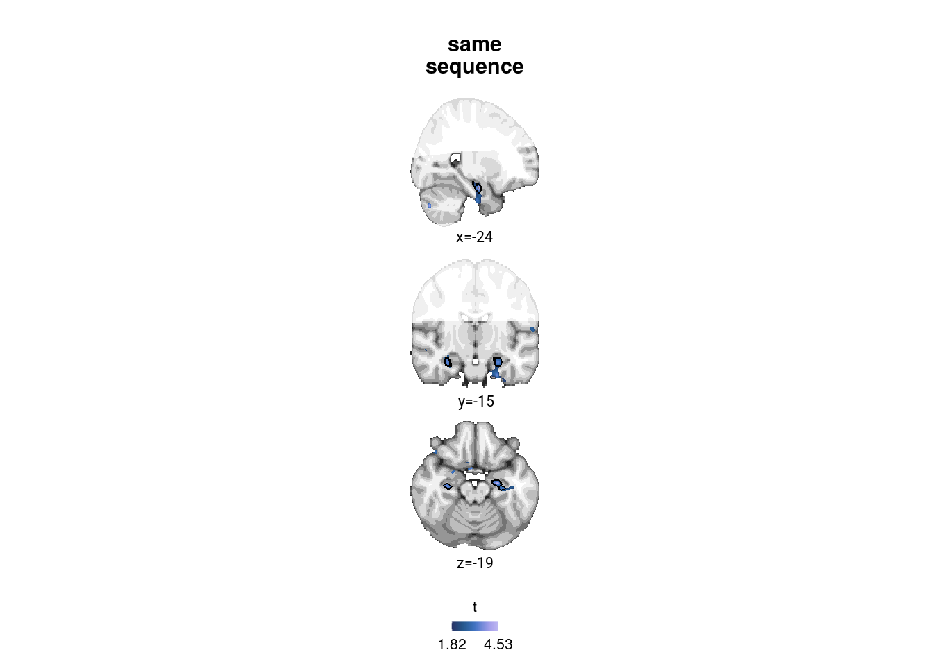
# save source data
file.copy(from = tvals_fn, to = file.path(dirs$source_dat_dir, "f7a.nii.gz"))
## [1] TRUEVirtual Time Across Sequences in Within-Searchlight Cluster
The plot above shows a significant effect of virtual time on pattern similarity change in some voxels of the hippocampus. To ask whether these voxels also show the across-sequence effect, we run an ROI-analyis based on the significant voxels from the within-searchlight (peak cluster from left hemisphere, defined at p<0.99 uncorrected within small volume correction mask). These data were calculated in the script virtem_mri_prepare_RSA_in_searchlight_cluster and are loaded here.
To test whether within- and across-sequence representations overlap, we defined an ROI based on the within-sequence searchlight analysis. Specifically, voxels belonging to the cluster around the peak voxel, thresholded at p<0.01 uncorrected within our small volume correction mask, were included. The analysis of representational change was then carried out as described for the other ROIs above.
Load data
# load the data
col_types_list <- cols_only(
        sub_id = col_character(),
        day1 = col_integer(), day2 = col_integer(),
        virtual_time1 = col_double(), virtual_time2 = col_double(),
        ps_change = col_double(), roi = col_factor())
fn <- file.path(dirs$data4analysis, "rsa_data_in_same-seq_searchlight_peak.txt")
rsa_dat_within_cluster <- as_tibble(read_csv(fn, col_types = col_types_list))
Prepare Time Metrics for RSA
Create day factor and create virtual temporal distance variables, analogous to main ROI analyses above.
# create predictors for RSA
rsa_dat_within_cluster <- rsa_dat_within_cluster %>%
  mutate(

    # pair of events from say or different day (dv = deviation code)
    same_day = day1 == day2,
    same_day_dv = plyr::mapvalues(same_day, from = c(FALSE, TRUE), to = c(-1, 1)),

    # absolute difference in time metrics
    vir_time_diff = abs(virtual_time1 - virtual_time2)) %>%

  # z-score the time metric predictors (within each subject)
  group_by(sub_id) %>%
  mutate_at(c("vir_time_diff"), scale, scale = TRUE) %>%
  ungroup()
Summary Statistics
First-level RSA
Let’s run the first-level analysis using virtual time as a predictor of pattern similarity change separately for each participant in this ROI.
set.seed(107) # set seed for reproducibility

# do RSA using linear model and calculate z-score for model fit based on permutations
rsa_fit_within_cluster <- rsa_dat_within_cluster %>% group_by(sub_id, same_day) %>%
          # run the linear model
          do(z = lm_perm_jb(in_dat = ., lm_formula = "ps_change ~ vir_time_diff", nsim = n_perm)) %>%
  mutate(z = list(setNames(z, c("z_intercept", "z_virtual_time")))) %>%
  unnest_wider(z)

# add group column used for plotting
rsa_fit_within_cluster$group <- factor(1)

# add a factor with character labels for within/across days and one to later color control in facets
rsa_fit_within_cluster <- rsa_fit_within_cluster %>%
  mutate(same_day_char = plyr::mapvalues(same_day,
                                         from = c(0, 1),
                                         to = c("across days", "within days"),
                                         warn_missing = FALSE),
         same_day_char = factor(same_day_char, levels = c("within days", "across days")))
Group Level
# run a group-level t-test on the different sequence RSA fits in the within-searchlight cluster
stats <- rsa_fit_within_cluster %>%
  filter(same_day == FALSE) %>%
  select(z_virtual_time) %>%
  paired_t_perm_jb (., n_perm = n_perm)

# Cohen's d with Hedges' correction for one sample using non-central t-distribution for CI
d<-cohen.d(d=(rsa_fit_within_cluster %>% filter(same_day == FALSE))$z_virtual_time,
           f=NA, paired=TRUE, hedges.correction=TRUE, noncentral=TRUE)
stats$d <- d$estimate
stats$dCI_low <- d$conf.int[[1]]
stats$dCI_high <- d$conf.int[[2]]

# print results
huxtable(stats) %>% theme_article()| estimate | statistic | p.value | p_perm | parameter | conf.low | conf.high | method | alternative | d | dCI_low | dCI_high |
|---|---|---|---|---|---|---|---|---|---|---|---|
| -0.424 | -2.19 | 0.037 | 0.0357 | 27 | -0.821 | -0.0275 | One Sample t-test | two.sided | -0.403 | -0.812 | -0.0251 |
Summary Statistics: t-test against 0 for virtual time across sequences in within-sequence searchlight peak
t27=-2.19, p=0.036, d=-0.40, 95% CI [-0.81, -0.03]
Lastly, we create a raincloud plot of the z-values
# select the data to plot
plot_dat <- rsa_fit_within_cluster %>% filter(same_day == FALSE)

f7b <- ggplot(plot_dat, aes(x=1, y=z_virtual_time, fill = group, color = group)) +
  gghalves::geom_half_violin(position=position_nudge(0.1),
                             side = "r", color = NA) +
  geom_point(aes(x = 0.8, y = z_virtual_time), alpha = 0.7,
             position = position_jitter(width = .1, height = 0),
             shape=16, size = 1) +
  geom_boxplot(position = position_nudge(x = 0, y = 0),
               width = .1, colour = "black", outlier.shape = NA) +
  stat_summary(fun = mean, geom = "point", size = 1, shape = 16,
               position = position_nudge(.1), colour = "black") +
  stat_summary(fun.data = mean_se, geom = "errorbar",
               position = position_nudge(.1), colour = "black", width = 0, size = 0.5)+
  scale_color_manual(values=unname(aHPC_colors["across_main"])) +
  scale_fill_manual(values=unname(aHPC_colors["across_main"])) +
  ylab('z RSA model fit') + xlab(element_blank()) +
  guides(fill = "none", color = "none") +
  annotate(geom = "text", x = 1, y = Inf, label = "*", hjust = 0.5, vjust = 1, size = 8/.pt, family=font2use) +
  ggtitle("\ndifferent sequence in\nsame sequence peak") +
  theme_cowplot() +
  theme(text = element_text(size=10), axis.text = element_text(size=8),
        legend.position = "none",
        axis.ticks.x = element_blank(), axis.text.x = element_blank())
f7b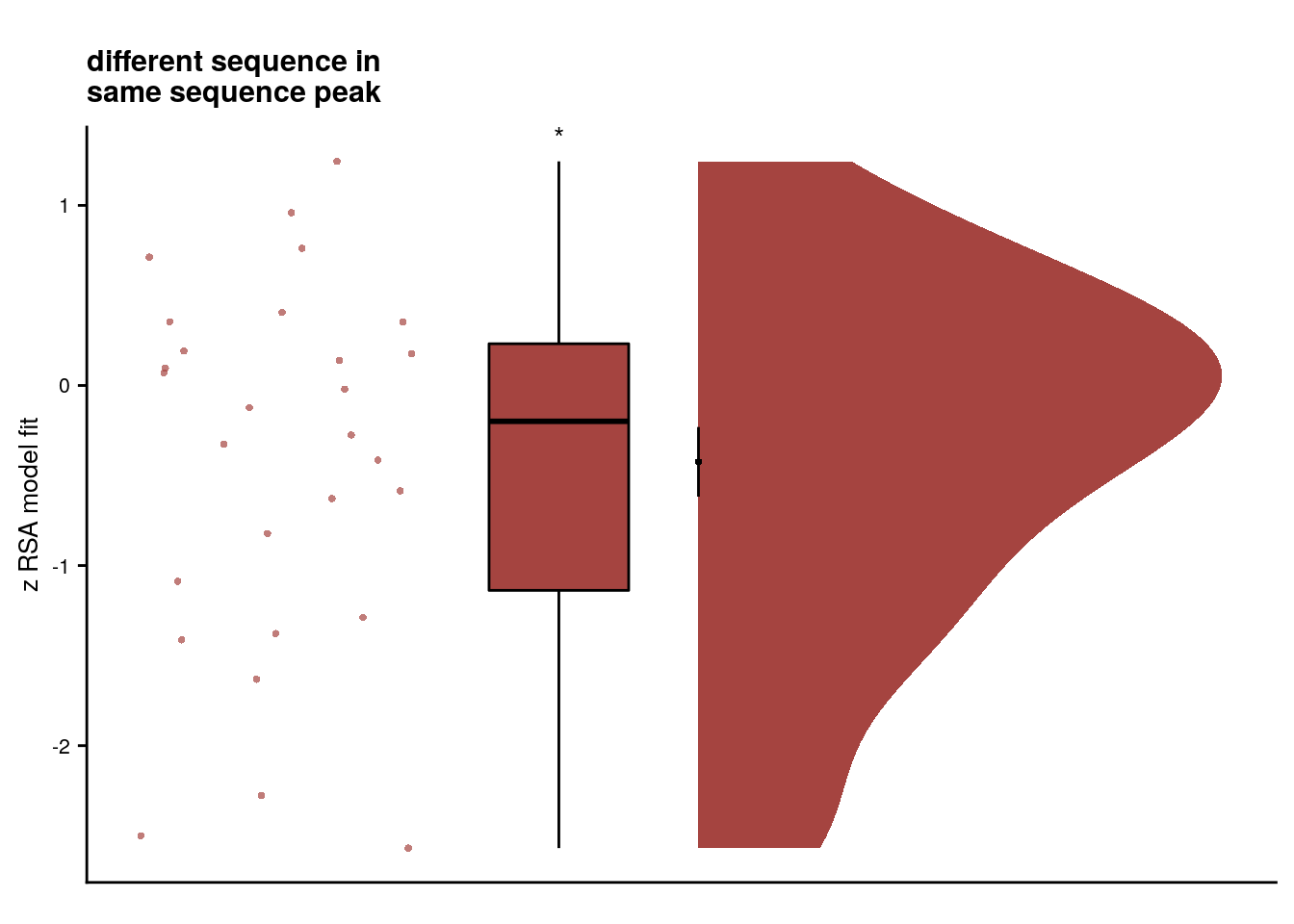
# save source data
source_dat <-ggplot_build(f7b)$data[[2]]
readr::write_tsv(source_dat %>% select(x,y),
                 file = file.path(dirs$source_dat_dir, "f7b.txt"))
Linear Mixed Effects
As for the main analyses, we also want to run the same model using linear mixed effects.
Due to singular fits we have to reduce the random effects structure until only random slopes are in the model.
# extract the comparisons from the same day
rsa_dat_diff_day <- rsa_dat_within_cluster %>% filter(same_day == FALSE)

# define the full model with virtual time difference as
# fixed effect and by-subject random slopes and random intercepts --> singular fit
formula <- "ps_change ~ vir_time_diff + (1 + vir_time_diff | sub_id)"
lmm_full <- lme4::lmer(formula, data = rsa_dat_diff_day, REML = FALSE)
## boundary (singular) fit: see ?isSingular# remove correlation --> still singular
formula <- "ps_change ~ vir_time_diff + (1 + vir_time_diff || sub_id)"
lmm_full <- lme4::lmer(formula, data = rsa_dat_diff_day, REML = FALSE)## boundary (singular) fit: see ?isSingular# only random slopes
set.seed(322) # set seed for reproducibility
formula <- "ps_change ~ vir_time_diff + (0 + vir_time_diff | sub_id)"
lmm_full <- lme4::lmer(formula, data = rsa_dat_diff_day, REML = FALSE)## boundary (singular) fit: see ?isSingularsummary(lmm_full, corr = FALSE)## Linear mixed model fit by maximum likelihood ['lmerMod']
## Formula: ps_change ~ vir_time_diff + (0 + vir_time_diff | sub_id)
## Data: rsa_dat_diff_day
##
## AIC BIC logLik deviance df.resid
## -23260.0 -23234.6 11634.0 -23268.0 4196
##
## Scaled residuals:
## Min 1Q Median 3Q Max
## -4.0842 -0.6392 0.0084 0.6616 3.7002
##
## Random effects:
## Groups Name Variance Std.Dev.
## sub_id vir_time_diff 0.0000000 0.00000
## Residual 0.0002299 0.01516
## Number of obs: 4200, groups: sub_id, 28
##
## Fixed effects:
## Estimate Std. Error t value
## (Intercept) -9.718e-05 2.343e-04 -0.415
## vir_time_diff -4.782e-04 2.341e-04 -2.043
## convergence code: 0
## boundary (singular) fit: see ?isSingular# tidy summary of the fixed effects that calculates 95% CIs
lmm_full_bm <- broom.mixed::tidy(lmm_full, effects = "fixed",
conf.int=TRUE, conf.method="profile",
optimizer = 'nloptwrap')## Computing profile confidence intervals ...# tidy summary of the random effects
lmm_full_bm_re <- broom.mixed::tidy(lmm_full, effects = "ran_pars")
# one way of testing for significance is by comparing the likelihood against a simpler model.
# Here, we drop the effect of virtual time difference and run an ANOVA. See e.g. Bodo Winter tutorial
set.seed(396) # set seed for reproducibility
formula <- "ps_change ~ 1 + (0 + vir_time_diff | sub_id)"
lmm_no_vir_time <- lme4::lmer(formula, data = rsa_dat_diff_day, REML = FALSE)
lmm_aov <-anova(lmm_no_vir_time, lmm_full)Mixed Model: Fixed effect of virtual time across sequences in within-sequence searchlight peak \(\chi^2\)(1)=4.13, p=0.042
Make mixed model summary table that includes overview of fixed and random effects as well as the model comparison to the nested (reduced) model.
fe_names <- c("intercept", "virtual time")
re_groups <- c(rep("participant",1), "residual")
re_names <- c("virtual time (SD)", "SD")
lmm_hux <- make_lme_huxtable(fix_df=lmm_full_bm,
ran_df = lmm_full_bm_re,
aov_mdl = lmm_aov,
fe_terms =fe_names,
re_terms = re_names,
re_groups = re_groups,
lme_form = gsub(" ", "", paste0(deparse(formula(lmm_full)),
collapse = "", sep="")),
caption = "Mixed Model: Virtual time explains representational change for different-sequence events in the peak cluster of the same-sequence searchlight analysis")
# convert the huxtable to a flextable for word export
stable_lme_same_seq_cluster_virtime_diff_seq <- convert_huxtable_to_flextable(ht = lmm_hux)
# print to screen
theme_article(lmm_hux)| fixed effects | ||||||
|---|---|---|---|---|---|---|
| term | estimate | SE | t-value | 95% CI | ||
| intercept | -0.000097 | 0.000234 | -0.41 | -0.000557 | 0.000362 | |
| virtual time | -0.000478 | 0.000234 | -2.04 | -0.000939 | -0.000018 | |
| random effects | ||||||
| group | term | estimate | ||||
| participant | virtual time (SD) | 0.000000 | ||||
| residual | SD | 0.015162 | ||||
| model comparison | ||||||
| model | npar | AIC | LL | X2 | df | p |
| reduced model | 3 | -23257.87 | 11631.93 | |||
| full model | 4 | -23260.00 | 11634.00 | 4.13 | 1 | 0.042 |
| model: ps_change~vir_time_diff+(0+vir_time_diff|sub_id); SE: standard error, CI: confidence interval, SD: standard deviation, npar: number of parameters, LL: log likelihood, df: degrees of freedom, corr.: correlation | ||||||
### PLOTS
lmm_full_bm <- lmm_full_bm %>%
mutate(term=as.factor(term))
# dot plot of Fixed Effect Coefficients with CIs
sfigmm_m <-ggplot(data = lmm_full_bm[2,], aes(x = term, color = term)) +
geom_hline(yintercept = 0, colour="black", linetype="dotted") +
geom_errorbar(aes(ymin = conf.low, ymax = conf.high, width = NA), size = 0.5) +
geom_point(aes(y = estimate), shape = 16, size = 1) +
scale_fill_manual(values = unname(aHPC_colors["across_main"])) +
scale_color_manual(values = unname(aHPC_colors["across_main"]),
labels = c("virtual time (diff. seq.)"), name = element_blank()) +
labs(x = element_blank(), y = "fixed effect\nestimate") +
guides(fill= "none", color=guide_legend(override.aes=list(fill=NA, alpha = 1, size=2, linetype=0))) +
annotate(geom = "text", x = 1, y = Inf, label = "*", hjust = 0.5, vjust = 1, size = 8/.pt, family=font2use) +
theme_cowplot() +
theme(legend.position = "none", axis.text.x=element_blank())
sfigmm_m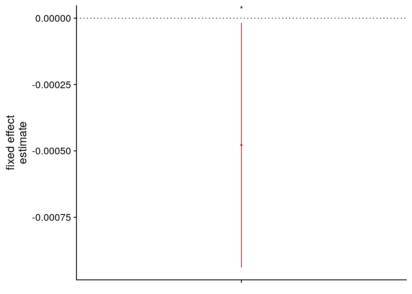
# estimate marginal means for each model term by omitting the terms argument
lmm_full_emm <- ggeffects::ggpredict(lmm_full, ci.lvl = 0.95) %>%
ggeffects::get_complete_df()
# plot marginal means
sfigmm_n <- ggplot(data = lmm_full_emm[lmm_full_emm$group == "vir_time_diff",], aes(color = group)) +
geom_line(aes(x, predicted)) +
geom_ribbon(aes(x, ymin = conf.low, ymax = conf.high, fill = group), alpha = .2, linetype=0) +
scale_color_manual(values = unname(aHPC_colors["across_main"]),
name = element_blank(), labels = "virtual time") +
scale_fill_manual(values = unname(aHPC_colors["across_main"])) +
ylab('estimated\nmarginal means') +
xlab('z virtual time') +
#ggtitle("Estimated marginal means") +
guides(fill = "none", color = "none") +
theme_cowplot() +
theme(legend.position = "none")
sfigmm_n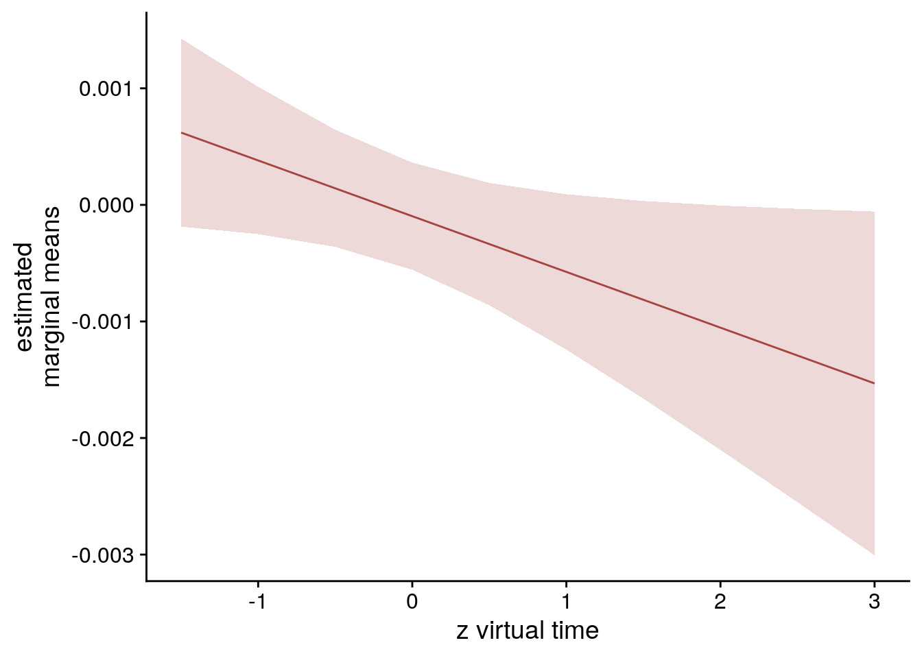
Virtual Time Across Sequences
Next, we plot the results of the searchlight looking at the across-sequence comparisons. This effect fails to reach the significance threshold when correcting for multiple comparisons. For visualization, we show the effect at p<0.05 uncorrected (within FOV). We report strongest cluster after small volume correction.
# read the cluster file for corrected results
fn <- file.path(dirs$data4analysis, "searchlight_results",
"diff_day_vir_time", "cluster_diff_day_vir_time_neg_svc_corrp_atlas.txt")
corrp_df <- readr::read_tsv(fn, col_types = c("ccdddddddddd"))
# print to screen
cat("no significant clusters in across-day virtual time (negative) searchlight:",
sprintf("\ncluster file has %d rows",
nrow(corrp_df)))## no significant clusters in across-day virtual time (negative) searchlight:
## cluster file has 0 rows# find and report peak voxel coordinates incl. p and t after SVC
corrp_fn <- file.path(dirs$data4analysis, "searchlight_results","diff_day_vir_time",
"diff_day_vir_time_neg_randomise_svc_fwhm3_tfce_corrp_tstat1.nii.gz")
corrp_nii <- readNIfTI2(corrp_fn)
coords <- which(corrp_nii == max(c(corrp_nii)), arr.ind = TRUE)
mnicoords <- vox2mni(coords)
tvals_fn <- file.path(dirs$data4analysis, "searchlight_results","diff_day_vir_time",
"diff_day_vir_time_neg_randomise_fov_fwhm3_tstat1.nii.gz")
t_nii <- readNIfTI2(tvals_fn)
cat("peak voxel in across-day virtual time (negative) searchlight:",
sprintf("\nx=%d, y=%d, z=%d, t=%.2f, corrected p =%.3f",
mnicoords[1], mnicoords[2], mnicoords[3],
-t_nii[coords[1], coords[2], coords[3]], 1-max(c(corrp_nii))))## peak voxel in across-day virtual time (negative) searchlight:
## x=-26, y=-19, z=-15, t=-3.96, corrected p =0.071Report additional clusters from exploratory analysis with threshold p<0.001 uncorrected and a minimum of 30 voxels per cluster.
# read the cluster file for uncorrected results
fn <- file.path(dirs$data4analysis, "searchlight_results",
"diff_day_vir_time", "cluster_diff_day_vir_time_neg_fov_uncorrp_atlas.txt")
uncorrp_df <- readr::read_tsv(fn, col_types = c("ccdddddddddd"))
# quick print
#uncorrp_df %>% huxtable::as_huxtable() %>% theme_article()
# add column with p-values (not 1-p as given by FSL) and manual labels
uncorrp_df <- uncorrp_df %>%
mutate(
t_extr = t_extr*-1, # multiply t-values by minus 1 because we tested the negative contrast
p = 1-max_1minusp,
atlas_label = c(
"cerebellum",
"cerebellum",
"lingual gyrus"
)) %>%
select(-c(max_1minusp, "Harvard_Oxford_Cortical", "Harvard_Oxford_Subcortical", cluster_index)) %>%
relocate(atlas_label)
# add p-values because small values are reported as 0 by FSL cluster
uncorrp_fn <- file.path(dirs$data4analysis, "searchlight_results","diff_day_vir_time",
"diff_day_vir_time_neg_randomise_fov_fwhm3_tfce_p_tstat1.nii.gz")
uncorrp_nii <- readNIfTI2(uncorrp_fn)
for (i in 1:nrow(uncorrp_df)){
coords <- mni2vox(c(uncorrp_df[i,]$x,uncorrp_df[i,]$y,uncorrp_df[i,]$z))
uncorrp_df[i,]$p <- 1-uncorrp_nii[coords[1], coords[2], coords[3]]
}Create pretty table that can be written to Word.
uncorrp_ht <- uncorrp_df %>%
as_huxtable() %>%
huxtable::set_contents(., row=1, value =c("Atlas Label", "Voxel Extent", "x", "y", "z", "COG x", "COG y", "COG z", "t", "p")) %>%
huxtable::insert_row(., rep("", ncol(.)), after=0) %>%
huxtable::merge_across(.,1,1:ncol(.)) %>%
huxtable::set_contents(., row=1, value ="Exploratory searchlight results, p-values uncorrected") %>%
huxtable::set_header_rows(.,row=1, value=TRUE) %>%
theme_article()
uncorrp_ht| Exploratory searchlight results, p-values uncorrected | |||||||||
|---|---|---|---|---|---|---|---|---|---|
| Atlas Label | Voxel Extent | x | y | z | COG x | COG y | COG z | t | p |
| cerebellum | 314 | 19 | -68 | -34 | 19.1 | -66.3 | -29.6 | -5.37 | 0.0002 |
| cerebellum | 104 | -1 | -68 | -14 | -1.86 | -69.1 | -14.3 | -3.44 | 0.0002 |
| lingual gyrus | 100 | -1 | -70 | 4 | -2.68 | -70.5 | 4.56 | -3.73 | 0.0002 |
stable_srchlght_diff_seq <- uncorrp_ht %>%
huxtable::add_footnote("x, y, z refer to MNI coordinates of minimum p-value in cluster, t denotes the most extreme t-value, COG: center of gravity", border = 0.5) %>%
huxtable::as_flextable() %>%
flextable::fontsize(size=10, part="all") %>%
flextable::font(fontname = font2use) %>%
flextable::style(i=c(1),
pr_c = officer::fp_cell(border.bottom = fp_border(),
border.top = fp_border())) %>%
flextable::bg(i=1, bg="lightgrey", part="all") %>%
flextable::padding(., padding = 3, part="all") %>% set_table_properties(., width=1, layout = "autofit") %>%
flextable::set_caption(., caption = "Searchlight Analysis: Virtual time explains representational change for different-sequence events",
style="Normal")# choose coordinates (these are chosen manually now) and get a data frame for labeling the plots
coords <- mni2vox(c(-25,-19,-15))
label_df <- data.frame(col_ind = sprintf("%s=%d",c("x","y","z"), vox2mni(coords)),
label = sprintf("%s=%d",c("x","y","z"), vox2mni(coords)))
# get ggplot object for template as background
ggTemplate<-getggTemplate(col_template=rev(RColorBrewer::brewer.pal(8, 'Greys')),brains=mni_nii,
all_brain_and_time_inds_one=TRUE,
mar=c(1,2,3), mar_ind=coords, row_ind = c(1,1,1),
col_ind=sprintf("%s=%d",c("x","y","z"),vox2mni(coords)), center_coords=TRUE)
# get uncorrected p-values in FOV
pfov_fn <- file.path(dirs$data4analysis, "searchlight_results","diff_day_vir_time",
"diff_day_vir_time_neg_randomise_fov_fwhm3_tfce_p_tstat1.nii.gz")
pfov_nii <- readNIfTI2(pfov_fn)
# t-values to plot (FOV)
tvals_fn <- file.path(dirs$data4analysis, "searchlight_results","diff_day_vir_time",
"diff_day_vir_time_neg_randomise_fov_fwhm3_tstat1.nii.gz")
t_nii <- readNIfTI2(tvals_fn)
# CAVE: because we are looking at the negative contrast, multiply the t-values by -1 to actually show
# negative t-values (they have previously been multiplied by -1 to run randomise, now revert this)
t_nii <- t_nii * -1
# threshold t-values for plotting
thresh <- 0.05
t_nii[pfov_nii < 1-thresh] <- NA
# get data frame for the t-values
t_df <- getBrainFrame(brains=t_nii, mar=c(1,2,3),
col_ind = sprintf("%s=%d",c("x","y","z"),vox2mni(coords)),
mar_ind=coords, mask=NULL, center_coords=TRUE)
f7c <- ggTemplate +
geom_tile(data=t_df, aes(x=row,y=col,fill=value))+
facet_wrap(~col_ind, nrow=3, ncol=1, strip.position = "top", scales = "free") +
scico::scale_fill_scico(palette = "lajolla",
begin = 0.3, end=0.9, direction = -1,
name = element_text("t"),
limits = round(range(t_df$value), digits=2),
breaks = round(range(t_df$value), digits=2)) +
ggtitle(label = "\ndifferent\nsequence") +
theme_cowplot(line_size = NA) +
theme(strip.background = element_blank(), strip.text.x = element_blank(),
plot.title = element_text(hjust = 0.5),
text = element_text(size=10), axis.text = element_text(size=8),
legend.text=element_text(size=8), legend.title = element_text(size=8),
legend.key.width = unit(0.01, "npc"),
legend.key.height = unit(0.015, "npc"),
legend.position = "bottom", legend.justification = c(0.5, 0),
aspect.ratio = 1)+
guides(fill = guide_colorbar(
direction = "horizontal",
title.position = "top",
title.hjust = 0.5,
label.position = "bottom"))+
xlab(element_blank()) + ylab(element_blank()) +
coord_cartesian(clip = "off") +
geom_text(data = label_df, x=0, y=c(-84.7,-70.37,-90.69), aes(label = label),
size = 8/.pt, family=font2use, vjust=1) +
# y coords found via command below (to keep text aligned across panels):
# ggplot_build(f6g)$layout$panel_scales_y[[2]]$range$range[1]-diff(ggplot_build(f6g)$layout$panel_scales_y[[2]]$range$range)/100*3
theme_no_ticks()
print(f7c)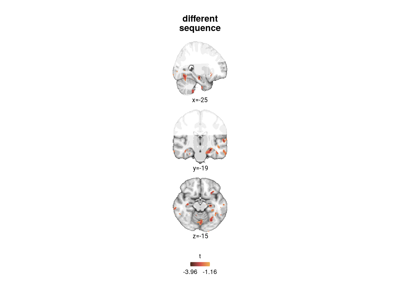
file.copy(from = tvals_fn, to = file.path(dirs$source_dat_dir, "f7c.nii.gz"))## [1] TRUEVisualization of Overlap
To visualize the overlap between the within- and the between-sequence effects we next create an overlap plot on a zoomed-in plot of the hippocampal region.
This is for visual purposes only, so we use a liberal threshold of p<0.05 within our small-volume-correction mask.
# choose coordinates (these are chosen manually now) and get a data frame for labeling the plots
coords <- mni2vox(c(-25,-18,-16))
label_df <- data.frame(col_ind = sprintf("%s=%d",c("x","y", "z"),vox2mni(coords)),
label = sprintf("%s=%d",c("x","y", "z"),vox2mni(coords)))
# for this plot we want to "zoom in", which we accomplish by masking out all but a small region of the brain
box2remove<-array(1, dim = dim(mni_nii))
box2remove[c(1:51, 131:182),,] <- 0
box2remove[,c(1:68, 150:218),] <- 0
box2remove[,,c(1:21, 101:182)] <- 0
mni_zoom_nii <- mni_nii * box2remove
mni_zoom_nii[mni_zoom_nii==0] <- NA
# get ggplot object for template as background
ggTemplate<-getggTemplate(col_template=rev(RColorBrewer::brewer.pal(8, 'Greys')),brains=mni_zoom_nii,
all_brain_and_time_inds_one=TRUE,
mar=c(1,2,3), mar_ind=coords, row_ind = c(1,1,1),
col_ind=sprintf("%s=%d",c("x","y","z"),vox2mni(coords)), center_coords=TRUE)
thresh <- 0.05
# get uncorrected p-values in FOV
fn <- file.path(dirs$data4analysis, "searchlight_results","same_day_vir_time",
"same_day_vir_time_randomise_svc_fwhm3_tfce_p_tstat1.nii.gz")
sameday_nii <- readNIfTI2(fn)
sameday_nii[sameday_nii > 1-thresh] = 1
sameday_nii[sameday_nii < 1-thresh] = 0
fn <- file.path(dirs$data4analysis, "searchlight_results","diff_day_vir_time",
"diff_day_vir_time_neg_randomise_svc_fwhm3_tfce_p_tstat1.nii.gz")
diffday_nii <- readNIfTI2(fn)
diffday_nii[diffday_nii > 1-thresh] = 2
diffday_nii[diffday_nii < 1-thresh] = 0
overlap_nii <- sameday_nii + diffday_nii
overlap_nii[overlap_nii < 1] = NA
# get data frame for the t-values
o_df <- getBrainFrame(brains=overlap_nii, mar=c(1,2,3),
col_ind = sprintf("%s=%d",c("x","y","z"),vox2mni(coords)),
mar_ind=coords, mask=NULL, center_coords=TRUE) %>%
mutate(value = as.factor(value), value = recode_factor(value, `1`="same", `2`="different", `3`="overlap"))
f7d <- ggTemplate +
geom_tile(data=o_df, aes(x=row,y=col,fill=value))+
facet_wrap(~col_ind, nrow=3, ncol=1, strip.position = "bottom", scales = "free") +
scale_fill_manual(values = unname(c(aHPC_colors["within_main"], aHPC_colors["across_main"], day_time_int_color)),
guide = guide_legend(override.aes=list(
alpha = 1, shape=16, size=2, linetype=0),
direction = "vertical",
title=element_blank(),
label.position = "right")) +
ggtitle(label = "\noverlap\n") +
theme_cowplot(line_size = NA) +
theme(strip.background = element_blank(), strip.text.x = element_blank(),
plot.title = element_text(hjust = 0.5),
text = element_text(size=10), axis.text = element_text(size=8),
legend.text=element_text(size=8), legend.title = element_text(size=8),
legend.key.size = unit(0.02, "npc"),
legend.position = "bottom", legend.justification = c(0.5, 0),
aspect.ratio = 1)+
xlab(element_blank()) + ylab(element_blank()) +
coord_cartesian(clip = "off") +
geom_text(data = label_df, x=0, y=c(-71.87,-67.75,-42.93), aes(label = label),
size = 8/.pt, family=font2use, vjust=1) +
# y coords found via command below (to keep text aligned across panels):
# ggplot_build(f6g)$layout$panel_scales_y[[2]]$range$range[1]-diff(ggplot_build(f6g)$layout$panel_scales_y[[2]]$range$range)/100*3
theme_no_ticks()
print(f7d)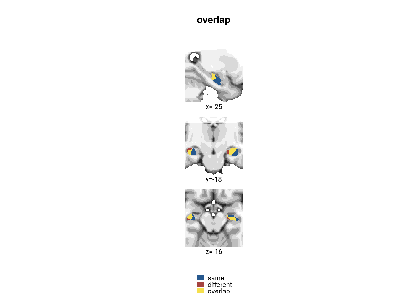
# save source data
overlap_nii[is.na(overlap_nii)] <- 0 # replace NAs with 0 to avoid trouble
writeNIfTI2(nim = overlap_nii, filename = file.path(dirs$source_dat_dir, "f7d"), dtype = TRUE)Virtual Time & Sequence Interaction
In our searchlight analyses, we also directly looked for voxels where the effect of virtual time differs depending on whether we are looking at events from the same sequence or from different sequences, i.e. an interaction of virtual temporal distances and a sequence factor (same/different).
Report significant clusters after small volume correction.
# read the cluster file for corrected results
fn <- file.path(dirs$data4analysis, "searchlight_results",
"day_time_interaction", "cluster_day_time_interaction_svc_corrp_atlas.txt")
corrp_df <- readr::read_tsv(fn, col_types = c("ccdddddddddd"))
# quick print
#corrp_df %>% huxtable::as_huxtable() %>% theme_article()
# add column with p-values (not 1-p as given by FSL) and manual labels
corrp_df <- corrp_df %>%
mutate(
p = 1-max_1minusp,
atlas_label = c("left hippocampus", "right hippocampus")) %>%
select(-c(max_1minusp, "Harvard_Oxford_Cortical", "Harvard_Oxford_Subcortical", cluster_index)) %>%
relocate(atlas_label)
# print to screen
cat("significant clusters in day-time interaction searchlight:",
sprintf("\n%s, peak voxel at x=%d, y=%d, z=%d; t=%.2f, corrected p=%.3f",
corrp_df$atlas_label, corrp_df$x, corrp_df$y, corrp_df$z, corrp_df$t_extr, corrp_df$p))## significant clusters in day-time interaction searchlight:
## left hippocampus, peak voxel at x=-26, y=-20, z=-15; t=4.15, corrected p=0.014
## right hippocampus, peak voxel at x=31, y=-16, z=-21; t=4.25, corrected p=0.007Report additional clusters from exploratory analysis with threshold p<0.001 uncorrected and a minimum of 30 voxels per cluster.
# read the cluster file for uncorrected results
fn <- file.path(dirs$data4analysis, "searchlight_results",
"day_time_interaction", "cluster_day_time_interaction_fov_uncorrp_atlas.txt")
uncorrp_df <- readr::read_tsv(fn, col_types = c("ccdddddddddd"))
# quick print
#uncorrp_df %>% huxtable::as_huxtable() %>% theme_article()
# add column with p-values (not 1-p as given by FSL) and manual labels
uncorrp_df <- uncorrp_df %>%
mutate(
p = 1-max_1minusp,
atlas_label = c(
"left hippocampus",
"right hippocampus",
"occipital pole",
"lingual gyrus",
"frontal pole",
"frontal pole",
"temporal fusiform cortex",
"intracalcarine sulcus")) %>%
select(-c(max_1minusp, "Harvard_Oxford_Cortical", "Harvard_Oxford_Subcortical", cluster_index)) %>%
filter(!str_detect(atlas_label, "hippocampus")) %>% # remove hippocampal clusters (already reported with SVC)
relocate(atlas_label)
# add p-values because small values are reported as 0 by FSL cluster
uncorrp_fn <- file.path(dirs$data4analysis, "searchlight_results","day_time_interaction",
"day_time_interaction_randomise_fov_fwhm3_tfce_p_tstat1.nii.gz")
uncorrp_nii <- readNIfTI2(uncorrp_fn)
for (i in 1:nrow(uncorrp_df)){
coords <- mni2vox(c(uncorrp_df[i,]$x,uncorrp_df[i,]$y,uncorrp_df[i,]$z))
uncorrp_df[i,]$p <- 1-uncorrp_nii[coords[1], coords[2], coords[3]]
}Make pretty overview table that can be saved to Word.
corrp_ht <- corrp_df %>%
as_huxtable() %>%
huxtable::set_contents(., row=1, value =c("Atlas Label", "Voxel Extent", "x", "y", "z", "COG x", "COG y", "COG z", "t", "p")) %>%
huxtable::insert_row(., rep("", ncol(.)), after=0) %>%
huxtable::merge_across(.,1,1:ncol(.)) %>%
huxtable::set_contents(., row=1, value ="Searchlight results in a priori regions of interest, p-values corrected using small volume correction") %>%
huxtable::set_header_rows(.,row=1, value=TRUE) %>%
theme_article()
corrp_ht| Searchlight results in a priori regions of interest, p-values corrected using small volume correction | |||||||||
|---|---|---|---|---|---|---|---|---|---|
| Atlas Label | Voxel Extent | x | y | z | COG x | COG y | COG z | t | p |
| left hippocampus | 359 | -26 | -20 | -15 | -23.4 | -15.5 | -18.6 | 4.15 | 0.014 |
| right hippocampus | 335 | 31 | -16 | -21 | 30.7 | -15.1 | -20.1 | 4.25 | 0.007 |
uncorrp_ht <- uncorrp_df %>%
as_huxtable() %>%
huxtable::set_contents(., row=1, value =c("Atlas Label", "Voxel Extent", "x", "y", "z", "COG x", "COG y", "COG z", "t", "p")) %>%
huxtable::insert_row(., rep("", ncol(.)), after=0) %>%
huxtable::merge_across(.,1,1:ncol(.)) %>%
huxtable::set_contents(., row=1, value ="Exploratory searchlight results, p-values uncorrected") %>%
huxtable::set_header_rows(.,row=1, value=TRUE) %>%
theme_article()
uncorrp_ht| Exploratory searchlight results, p-values uncorrected | |||||||||
|---|---|---|---|---|---|---|---|---|---|
| Atlas Label | Voxel Extent | x | y | z | COG x | COG y | COG z | t | p |
| occipital pole | 103 | 17 | -91 | -8 | 17.7 | -90.6 | -6.62 | 4.08 | 0.0002 |
| lingual gyrus | 102 | -5 | -73 | 5 | -3.59 | -70.4 | 5.01 | 3.72 | 0.0002 |
| frontal pole | 96 | 43 | 43 | 18 | 45.4 | 43.4 | 19.7 | 4.31 | 0.0006 |
| frontal pole | 45 | 35 | 43 | 17 | 37 | 43.2 | 18.5 | 3.81 | 0.0006 |
| temporal fusiform cortex | 40 | -25 | -10 | -45 | -25.3 | -10.3 | -42.9 | 3.14 | 0.0004 |
| intracalcarine sulcus | 33 | -4 | -77 | 11 | -2.85 | -75.8 | 11.5 | 3.56 | 0.0002 |
stable_srchlght_interaction <- rbind(corrp_ht, uncorrp_ht) %>%
huxtable::add_footnote("x, y, z refer to MNI coordinates of minimum p-value in cluster, t denotes the most extreme t-value, COG: center of gravity", border = 0.5) %>%
huxtable::as_flextable() %>%
flextable::fontsize(size=10, part="all") %>%
flextable::font(fontname = font2use) %>%
flextable::style(i=c(1,nrow(corrp_ht)+1),
pr_c = officer::fp_cell(border.bottom = fp_border(),
border.top = fp_border())) %>%
flextable::bg(i=c(1,nrow(corrp_ht)+1), bg="lightgrey", part="all") %>%
flextable::padding(., padding = 3, part="all") %>%
flextable::set_table_properties(., width=1, layout = "autofit") %>%
flextable::set_caption(., caption = "Searchlight Analysis: Interaction of virtual time and sequence membership",
style="Normal")As for the within-day effect, we show the t-values at p<0.01 uncorrected (based on field of view) and outline voxels surviving corrections (small volume correction) in black.
# choose coordinates (these are chosen manually now) and get a data frame for labeling the plots
coords <- mni2vox(c(31,-15,-19))
label_df <- data.frame(col_ind = sprintf("%s=%d",c("x","y", "z"),vox2mni(coords)),
label = sprintf("%s=%d",c("x","y", "z"),vox2mni(coords)))
# get ggplot object for template as background
ggTemplate<-getggTemplate(col_template=rev(RColorBrewer::brewer.pal(8, 'Greys')),brains=mni_nii,
all_brain_and_time_inds_one=TRUE,
mar=c(1,2,3), mar_ind=coords, row_ind = c(1,1,1),
col_ind=sprintf("%s=%d",c("x","y","z"),vox2mni(coords)), center_coords=TRUE)
# get uncorrected p-values in FOV
pfov_fn <- file.path(dirs$data4analysis, "searchlight_results","day_time_interaction",
"day_time_interaction_randomise_fov_fwhm3_tfce_p_tstat1.nii.gz")
pfov_nii <- readNIfTI2(pfov_fn)
# t-values to plot (FOV)
tvals_fn <- file.path(dirs$data4analysis, "searchlight_results","day_time_interaction",
"day_time_interaction_randomise_fov_fwhm3_tstat1.nii.gz")
t_nii <- readNIfTI2(tvals_fn)
# threshold t-values for plotting
thresh <- 0.01
t_nii[pfov_nii < 1-thresh] <- NA
# get data frame for the t-values
t_df <- getBrainFrame(brains=t_nii, mar=c(1,2,3),
col_ind = sprintf("%s=%d",c("x","y","z"),vox2mni(coords)),
mar_ind=coords, mask=NULL, center_coords=TRUE)
# load outline
outl_fn <- file.path(dirs$data4analysis, "searchlight_results","day_time_interaction",
"day_time_interaction_randomise_svc_fwhm3_tfce_corrp_outline.nii.gz")
outl_nii <- readNIfTI2(outl_fn)
# remove zero voxels and get dataframe at coordinates
outl_nii[outl_nii == 0] <- NA
o_df <- getBrainFrame(brains=outl_nii, mar=c(1,2,3),
col_ind = sprintf("%s=%d",c("x","y","z"),vox2mni(coords)),
mar_ind=coords, mask=NULL, center_coords=TRUE)
f7e <- ggTemplate +
geom_tile(data=t_df, aes(x=row,y=col,fill=value))+
geom_tile(data=o_df, aes(x=row,y=col), fill="black")+
facet_wrap(~col_ind, nrow=3, ncol=1, strip.position = "bottom", scales = "free") +
scico::scale_fill_scico(palette = "buda",
begin = 0, end=1,
name = element_text("t"),
limits = round(range(t_df$value), digits=2),
breaks = round(range(t_df$value), digits=2)) +
ggtitle(label = "\nsame vs.\ndifferent") +
theme_cowplot(line_size = NA) +
theme(strip.background = element_blank(), strip.text.x = element_blank(),
plot.title = element_text(hjust = 0.5),
text = element_text(size=10), axis.text = element_text(size=8),
legend.text=element_text(size=8), legend.title = element_text(size=8),
legend.key.width = unit(0.01, "npc"),
legend.key.height = unit(0.015, "npc"),
legend.position = "bottom", legend.justification = c(0.5, 0),
aspect.ratio = 1)+
guides(fill = guide_colorbar(
direction = "horizontal",
title.position = "top",
title.hjust = 0.5,
label.position = "bottom"))+
xlab(element_blank()) + ylab(element_blank()) +
coord_cartesian(clip = "off") +
geom_text(data = label_df, x=0, y=c(-84.64,-67.25,-86.51), aes(label = label),
size = 8/.pt, family=font2use, vjust=1) +
# y coords found via command below (to keep text aligned across panels):
# ggplot_build(f6g)$layout$panel_scales_y[[2]]$range$range[1]-diff(ggplot_build(f6g)$layout$panel_scales_y[[2]]$range$range)/100*3
theme_no_ticks()
print(f7e)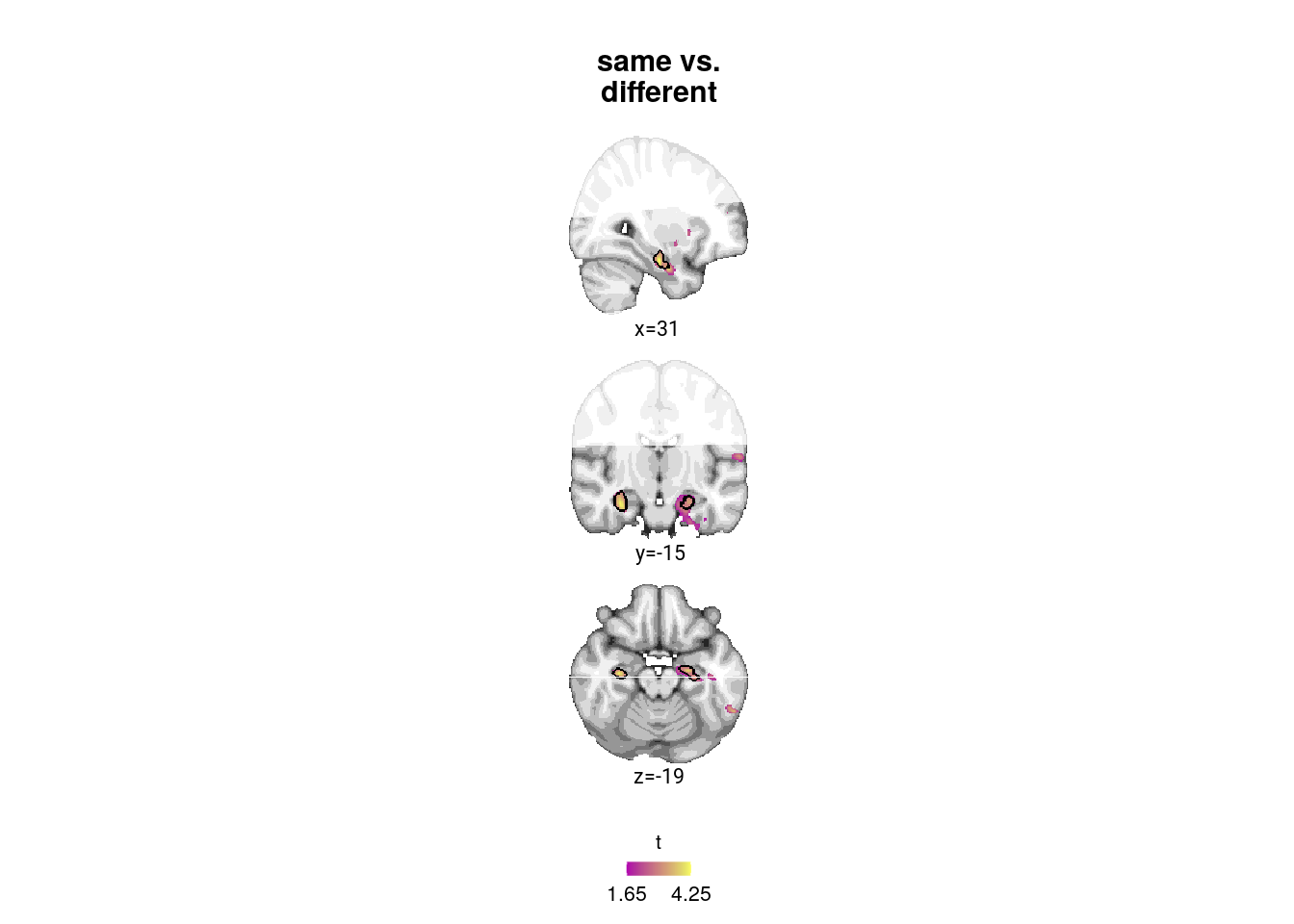
file.copy(from = tvals_fn, to = file.path(dirs$source_dat_dir, "f7e.nii.gz"))## [1] TRUELet’s compose figure 7.
layout <- "ABCDE"
f7 <- f7a+f7b+f7c+f7d+f7e +
plot_layout(design = layout, guides = "keep") &
plot_annotation(theme = theme(plot.margin = margin(t=0, r=-8, b=0, l=-19, unit="pt")),
tag_levels = 'A') &
theme(legend.text=element_text(size=8),
legend.title=element_text(size=8),
plot.tag = element_text(size = 10, face="bold"),
text = element_text(size=10, family=font2use),
plot.title = element_text(family=font2use, size=10, face="plain"))
f7[[1]] <- f7[[1]] +
theme(plot.tag = element_text(margin = margin(l =13)))
# save and print
fn <- here("figures", "f7")
ggsave(paste0(fn, ".pdf"), plot=f7, units = "cm",
width = 18, height = 12, dpi = "retina", device = cairo_pdf)
ggsave(paste0(fn, ".png"), plot=f7, units = "cm",
width = 18, height = 12, dpi = "retina", device = "png")
Figure 7. Overlapping representations of within- and across-sequence relations. A. Searchlight analysis results show a positive relationship between representational change and virtual temporal distances for event pairs from the same sequence in the bilateral anterior hippocampus. Statistical image is thresholded at puncorrected<0.01; voxels within black outline are significant after correction for multiple comparisons using small volume correction. B. In the peak cluster from the independent within-sequence searchlight analysis (A), representational change was negatively related to virtual temporal distances between events from different sequences. Circles show individual participant Z-values from summary statistics approach; boxplot shows median and upper/lower quartile along with whiskers extending to most extreme data point within 1.5 interquartile ranges above/below the upper/lower quartile; black circle with error bars corresponds to mean±S.E.M.; distribution shows probability density function of data points. C. Searchlight analysis results show negative relationship between representational change and temporal distances for different-sequence event pairs. Statistical image is thresholded at puncorrected <0.05. D. Within the anterior hippocampus, the effects for events from the same sequence and from two different sequences overlap. Visualization is based on statistical images thresholded at puncorrected <0.05 within small volume correction mask. E. Searchlight analysis results show a bilateral interaction effect in the anterior hippocampus that is defined by a differential relationship of virtual temporal distances and representational change for events from the same and different sequences. Statistical image is thresholded at puncorrected<0.01; voxels within black outline are significant after correction for multiple comparisons using small volume correction. A, C-E. Results are shown on the MNI template with voxels outside the field of view displayed in lighter shades of gray. See Supplemental Figure 9 for additional exploratory results. * p<0.05
Exploratory Searchlight Results
Further, we used a liberal threshold of puncorrected<0.001 to explore the data for additional effects within our field of view. Exploratory searchlight results are shown in Supplemental Figure 9 and clusters with a minimum extent of 30 voxels are listed in Supplemental Tables 12, 14 and 15.
For completeness, let’s create a supplemental figure that shows the additional clusters outside of our a priori regions of interest.
Same Sequence
# choose coordinates (these are chosen manually now) and get a data frame for labeling the plots
mni_coords <- c(48, 6, -13)
coords <- c(mni2vox(c(48,NA,NA))[1], mni2vox(c(6,NA,NA))[1], mni2vox(c(NA,-13,NA))[2])
label_df <- data.frame(col_ind = sprintf("%s=%d",c("x","x", "y"),mni_coords),
label = sprintf("%s=%d",c("x","x", "y"),mni_coords))
# get ggplot object for template as background
ggTemplate<-getggTemplate(col_template=rev(RColorBrewer::brewer.pal(8, 'Greys')),brains=mni_nii,
all_brain_and_time_inds_one=TRUE,
mar=c(1,1,2), mar_ind=coords, row_ind = c(1,1,1),
col_ind=sprintf("%s=%d",c("x","x","y"),mni_coords), center_coords=TRUE)
# get uncorrected p-values in FOV
pfov_fn <- file.path(dirs$data4analysis, "searchlight_results","day_time_interaction",
"day_time_interaction_randomise_fov_fwhm3_tfce_p_tstat1.nii.gz")
pfov_nii <- readNIfTI2(pfov_fn)
# t-values to plot (FOV)
tvals_fn <- file.path(dirs$data4analysis, "searchlight_results","day_time_interaction",
"day_time_interaction_randomise_fov_fwhm3_tstat1.nii.gz")
t_nii <- readNIfTI2(tvals_fn)
# threshold t-values for plotting
thresh <- 0.01
t_nii[pfov_nii < 1-thresh] <- NA
# get data frame for the t-values
t_df <- getBrainFrame(brains=t_nii, mar=c(1,1,2),
col_ind = sprintf("%s=%d",c("x","x","y"),mni_coords),
mar_ind=coords, mask=NULL, center_coords=TRUE)
sfiga_srchlght <- ggTemplate +
geom_tile(data=t_df, aes(x=row,y=col,fill=value))+
facet_wrap(~col_ind, nrow=3, ncol=1, strip.position = "top", scales = "free") +
scico::scale_fill_scico(palette = "devon",
begin = 0.1, end=0.7,
name = element_text("t"),
limits = round(range(t_df$value), digits=2),
breaks = round(range(t_df$value), digits=2)) +
ggtitle(label = "\nsame\nsequence") +
theme_cowplot(line_size = NA) +
theme(strip.background = element_blank(), strip.text.x = element_blank(),
plot.title = element_text(hjust = 0.5),
text = element_text(size=10), axis.text = element_text(size=8),
legend.text=element_text(size=8), legend.title = element_text(size=8),
legend.key.width = unit(0.02, "npc"),
legend.key.height = unit(0.015, "npc"),
legend.position = "bottom", legend.justification = c(0.5, 0),
aspect.ratio = 1)+
guides(fill = guide_colorbar(
direction = "horizontal",
title.position = "top",
title.hjust = 0.5,
label.position = "bottom"))+
xlab(element_blank()) + ylab(element_blank()) +
coord_cartesian(clip = "off") +
geom_text(data = label_df, x=0, y=c(-77.13,-94.03,-68.28), aes(label = label),
size = 8/.pt, family=font2use, vjust=1) +
# y coords found via command below (to keep text aligned across panels):
# ggplot_build(f6g)$layout$panel_scales_y[[2]]$range$range[1]-diff(ggplot_build(f6g)$layout$panel_scales_y[[2]]$range$range)/100*3
theme_no_ticks()
print(sfiga_srchlght)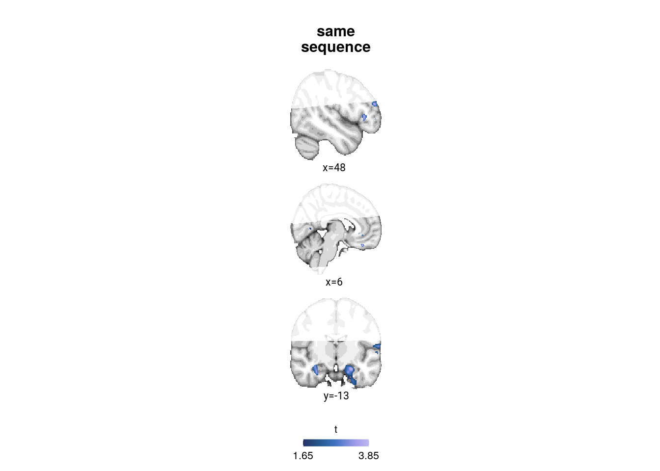
Different Sequence
# choose coordinates (these are chosen manually now) and get a data frame for labeling the plots
mni_coords <- c(-2, 19, -70)
coords <- c(mni2vox(c(-2,NA,NA))[1],
mni2vox(c(19,NA,NA))[1],
mni2vox(c(NA,-70,NA))[2])
label_df <- data.frame(col_ind = sprintf("%s=%d",c("x","x","y"),mni_coords),
label = sprintf("%s=%d",c("x","x","y"),mni_coords))
# get ggplot object for template as background
ggTemplate<-getggTemplate(col_template=rev(RColorBrewer::brewer.pal(8, 'Greys')),brains=mni_nii,
all_brain_and_time_inds_one=TRUE,
mar=c(1,1,2), mar_ind=coords, row_ind = c(1,1,1),
col_ind=sprintf("%s=%d",c("x","x","y"),mni_coords), center_coords=TRUE)
# get uncorrected p-values in FOV
pfov_fn <- file.path(dirs$data4analysis, "searchlight_results","diff_day_vir_time",
"diff_day_vir_time_neg_randomise_fov_fwhm3_tfce_p_tstat1.nii.gz")
pfov_nii <- readNIfTI2(pfov_fn)
# t-values to plot (FOV)
tvals_fn <- file.path(dirs$data4analysis, "searchlight_results","diff_day_vir_time",
"diff_day_vir_time_neg_randomise_fov_fwhm3_tstat1.nii.gz")
t_nii <- readNIfTI2(tvals_fn)
# threshold t-values for plotting
thresh <- 0.01
t_nii[pfov_nii < 1-thresh] <- NA
# get data frame for the t-values
t_df <- getBrainFrame(brains=t_nii, mar=c(1,1,2),
col_ind = sprintf("%s=%d",c("x","x","y"),mni_coords),
mar_ind=coords, mask=NULL, center_coords=TRUE)
sfigb_srchlght <- ggTemplate +
geom_tile(data=t_df, aes(x=row,y=col,fill=value))+
facet_wrap(~col_ind, nrow=3, ncol=1, strip.position = "top", scales = "free") +
scico::scale_fill_scico(palette = "lajolla",
begin = 0.3, end=0.9, direction = -1,
name = element_text("t"),
limits = round(range(t_df$value), digits=2),
breaks = round(range(t_df$value), digits=2)) +
ggtitle(label = "\ndifferent\nsequence") +
theme_cowplot(line_size = NA) +
theme(strip.background = element_blank(), strip.text.x = element_blank(),
plot.title = element_text(hjust = 0.5),
text = element_text(size=10), axis.text = element_text(size=8),
legend.text=element_text(size=8), legend.title = element_text(size=8),
legend.key.width = unit(0.02, "npc"),
legend.key.height = unit(0.015, "npc"),
legend.position = "bottom", legend.justification = c(0.5, 0),
aspect.ratio = 1)+
guides(fill = guide_colorbar(
direction = "horizontal",
title.position = "top",
title.hjust = 0.5,
label.position = "bottom"))+
xlab(element_blank()) + ylab(element_blank()) +
coord_cartesian(clip = "off") +
geom_text(data = label_df, x=0, y=c(-93.97,-84.79,-82.34), aes(label = label),
size = 8/.pt, family=font2use, vjust=1) +
# y coords found via command below (to keep text aligned across panels):
# ggplot_build(f6g)$layout$panel_scales_y[[2]]$range$range[1]-diff(ggplot_build(f6g)$layout$panel_scales_y[[2]]$range$range)/100*3
theme_no_ticks()
print(sfigb_srchlght)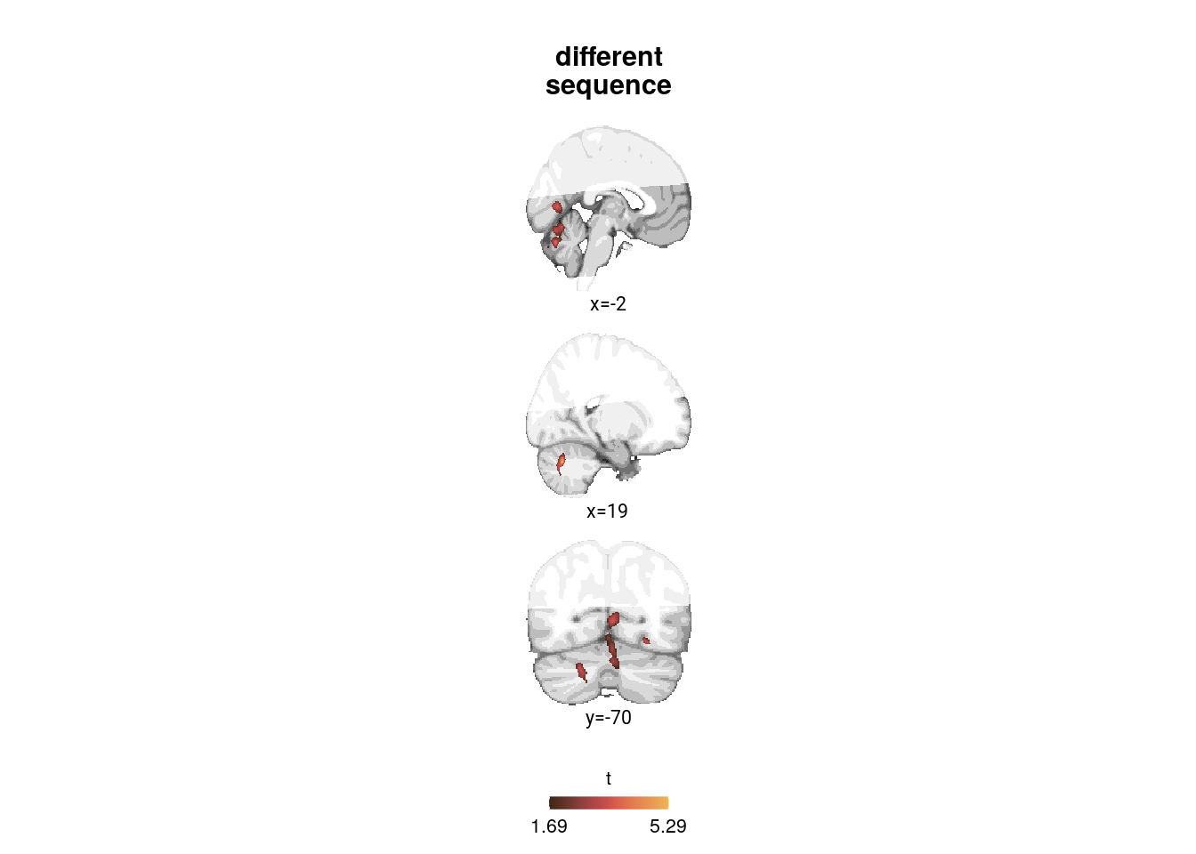
Virtual Time and Sequence Interaction
# choose coordinates (these are chosen manually now) and get a data frame for labeling the plots
mni_coords <- c(-4,17,20)
coords <- c(mni2vox(c(-4,NA,NA))[1],
mni2vox(c(17,NA,NA))[1],
mni2vox(c(NA,NA,20))[3])
label_df <- data.frame(col_ind = sprintf("%s=%d",c("x","x","z"),mni_coords),
label = sprintf("%s=%d",c("x","x","z"),mni_coords))
# get ggplot object for template as background
ggTemplate<-getggTemplate(col_template=rev(RColorBrewer::brewer.pal(8, 'Greys')),brains=mni_nii,
all_brain_and_time_inds_one=TRUE,
mar=c(1,1,3), mar_ind=coords, row_ind = c(1,1,1),
col_ind=sprintf("%s=%d",c("x","x","z"),mni_coords), center_coords=TRUE)
# get uncorrected p-values in FOV
pfov_fn <- file.path(dirs$data4analysis, "searchlight_results","day_time_interaction",
"day_time_interaction_randomise_fov_fwhm3_tfce_p_tstat1.nii.gz")
pfov_nii <- readNIfTI2(pfov_fn)
# t-values to plot (FOV)
tvals_fn <- file.path(dirs$data4analysis, "searchlight_results","day_time_interaction",
"day_time_interaction_randomise_fov_fwhm3_tstat1.nii.gz")
t_nii <- readNIfTI2(tvals_fn)
# threshold t-values for plotting
thresh <- 0.01
t_nii[pfov_nii < 1-thresh] <- NA
# get data frame for the t-values
t_df <- getBrainFrame(brains=t_nii, mar=c(1,1,3),
col_ind = sprintf("%s=%d",c("x","x","z"),mni_coords),
mar_ind=coords, mask=NULL, center_coords=TRUE)
sfigc_srchlght <- ggTemplate +
geom_tile(data=t_df, aes(x=row,y=col,fill=value))+
facet_wrap(~col_ind, nrow=3, ncol=1, strip.position = "bottom", scales = "free") +
scico::scale_fill_scico(palette = "buda",
begin = 0, end=1,
name = element_text("t"),
limits = round(range(t_df$value), digits=2),
breaks = round(range(t_df$value), digits=2)) +
ggtitle(label = "\nsame vs.\ndifferent") +
theme_cowplot(line_size = NA) +
theme(strip.background = element_blank(), strip.text.x = element_blank(),
plot.title = element_text(hjust = 0.5),
text = element_text(size=10), axis.text = element_text(size=8),
legend.text=element_text(size=8), legend.title = element_text(size=8),
legend.key.width = unit(0.02, "npc"),
legend.key.height = unit(0.015, "npc"),
legend.position = "bottom", legend.justification = c(0.5, 0),
aspect.ratio = 1)+
guides(fill = guide_colorbar(
direction = "horizontal",
title.position = "top",
title.hjust = 0.5,
label.position = "bottom"))+
xlab(element_blank()) + ylab(element_blank()) +
coord_cartesian(clip = "off") +
geom_text(data = label_df, x=0, y=c(-94,-86.85,-88.66), aes(label = label),
size = 8/.pt, family=font2use, vjust=1) +
# y coords found via command below (to keep text aligned across panels):
# ggplot_build(f6g)$layout$panel_scales_y[[2]]$range$range[1]-diff(ggplot_build(f6g)$layout$panel_scales_y[[2]]$range$range)/100*3
theme_no_ticks()
print(sfigc_srchlght)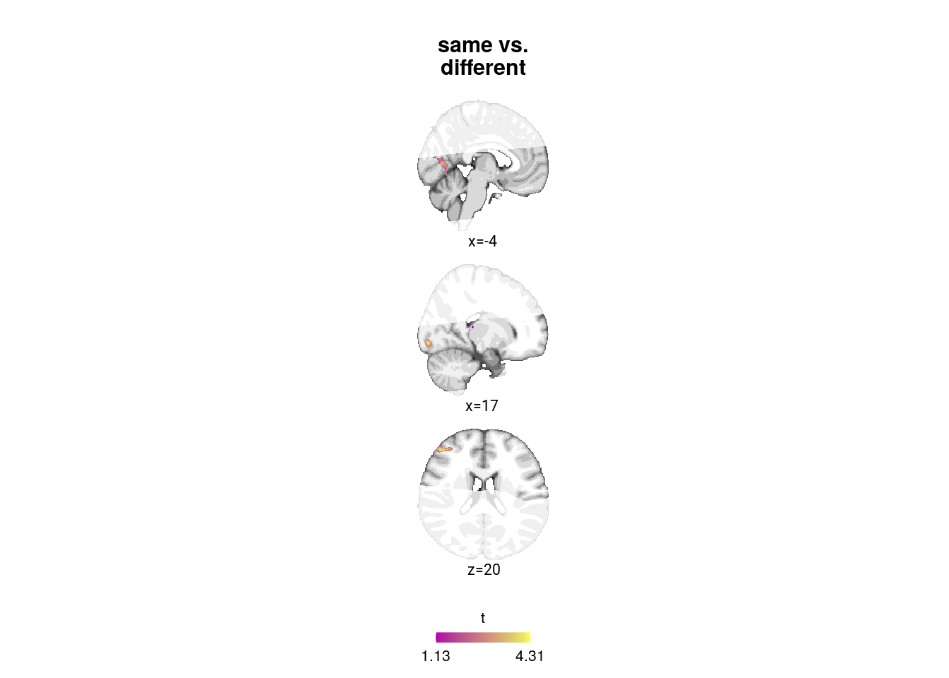
Overview Figure
layout="
ABC
ABC
ABC"
sfig_srchlght <- sfiga_srchlght + sfigb_srchlght + sfigc_srchlght +
plot_layout(design = layout, guides = "keep") &
plot_annotation(theme = theme(plot.margin = margin(t=0, r=-9, b=0, l=-19, unit="pt")),
tag_levels = 'A') &
theme(plot.tag = element_text(size = 10, face="bold"),
legend.text=element_text(size=8),
legend.title=element_text(size=8),
text = element_text(size=10, family=font2use),
plot.title = element_text(family=font2use, size=10, face="plain"))
sfig_srchlght[[1]] <- sfig_srchlght[[1]] +
theme(plot.tag = element_text(margin = margin(l=19)))
# save and print
fn <- here("figures", "sf09")
ggsave(paste0(fn, ".pdf"), plot=sfig_srchlght, units = "cm",
width = 8.5, height = 10, dpi = "retina", device = cairo_pdf)
ggsave(paste0(fn, ".png"), plot=sfig_srchlght, units = "cm",
width = 8.5, height = 10, dpi = "retina", device = "png")
Supplemental Figure 9. Exploratory searchlight results. A. For same-sequence event pairs, clusters of voxels in which pattern similarity change correlated positively with temporal distances were detected in the frontal pole, frontal medial cortex and left entorhinal cortex (see Supplemental Table 12). B. Pattern similarity change correlated negatively with temporal distances between events from different sequences in the cerebellum and lingual gyrus (see Supplemental Table 14). C. The interaction effect, defined as correlations of temporal distances and pattern similarity change depending on whether pairs of events belonged to the same sequence or not, was observed in the occipital pole, lingual gyrus, frontal pole, temporal fusiform cortex and the intracalcerine sulcus (see Supplemental Table 15). A-C. Statistical images are thresholded at p<0.01 uncorrected for display purposes. No clusters outside the hippocampal-entorhinal region survived corrections for multiple comparisons.
8.12 Correlation of behavioral generalization bias with searchlight effects
We want to see whether the structure generalization bias in behavior relates to the RSA effects For that, we extract the t-value of the searchlight effect at the peak voxel for each participant and run Spearman correlations.
We then asked whether the deviation between the average time of other events and an event’s true virtual time was systematically related to signed errors in constructed event times. A positive relationship between the relative time of other events and time construction errors indicates that, when other events at the same sequence position are relatively late, participants are biased to construct a later time for a given event than when the other events took place relatively early. In the summary statistics approach, we ran a linear regression for each participant (Figure 8B, Supplemental Figure 10A) and tested the resulting coefficients for statistical significance using the permutation-based procedures described above (Figure 8C). The regression coefficients from this approach were used to test for a relationship between the behavioral generalization bias and the hippocampal searchlight effects (see below).
Correlation with across-sequence searchlight effect
We start with the across-sequence searchlight effect. Note that the t-values are more negative for those subjects who show a stronger effect, so we might expect a negative correlation: Participants with stronger across-sequence generalization in the hippocampus could more strongly be biased by the abstracted structure in their specific constructions.
# load the p-values from across-sequence searchlight (SVC corrected)
p_fn <- file.path(dirs$data4analysis, "searchlight_results","diff_day_vir_time",
"diff_day_vir_time_neg_randomise_svc_fwhm3_tfce_corrp_tstat1.nii.gz")
p_nii <- readNIfTI2(p_fn)
# load the 4D image with searchlight t-values for each participant
tvals_fn <- file.path(dirs$data4analysis, "searchlight_results","diff_day_vir_time",
"diff_day_vir_time_4d_smooth_fwhm3.nii.gz")
t_nii <- readNIfTI2(tvals_fn)
# find the coordinates of peak voxel
coords<-which(p_nii ==max(p_nii))
# store the searchlight t-value for each subject at this voxel
fit_beh_bias <- fit_beh_bias %>% add_column(srchlght_across_t=NA)
for (i in 1:28){
curr_nii <- t_nii[,,,i]
fit_beh_bias$srchlght_across_t[i] <- mean(curr_nii[cbind(coords)])
}
# correlate the same-sequence searchlight effect with the behavioral bias
stats <- tidy(cor.test(fit_beh_bias$beta_rel_time_other_events, fit_beh_bias$srchlght_across_t,
method="spearman"))
# print results
huxtable(stats) %>% theme_article() | estimate | statistic | p.value | method | alternative |
|---|---|---|---|---|
| -0.194 | 4.36e+03 | 0.322 | Spearman's rank correlation rho | two.sided |
Spearman correlation of across-sequence searchlight effect in aHPC and behavioral generalization bias: r=-0.19, p=0.322
The effect is not significant, but let’s still visualize it as a scatter plot.
# scatterplot
f8e <- ggplot(fit_beh_bias, aes(x=srchlght_across_t, y=beta_rel_time_other_events))+
geom_point(size = 1, shape = 16) +
geom_smooth(method='lm', formula= y~x,
colour=unname(aHPC_colors["across_main"]),
fill=unname(aHPC_colors["across_main"]),
size=1)+
scale_x_continuous(labels = c(-1.5, -1, -0.5, 0, 0.5, 1)) +
xlab("diff. sequence\nsearchlight (t)") +
ylab("behavioral bias") +
annotate("text", x=Inf, y=Inf, hjust=1,vjust=1,
size = 6/.pt, family = font2use,
label=sprintf("r=%.2f\np=%.3f",
round(stats$estimate,2), round(stats$p.value, 3)))+
theme_cowplot() +
theme(text = element_text(size=10, family=font2use),
axis.text = element_text(size=8),
legend.text=element_text(size=8),
legend.title=element_text(size=8),
legend.position = "none")
f8e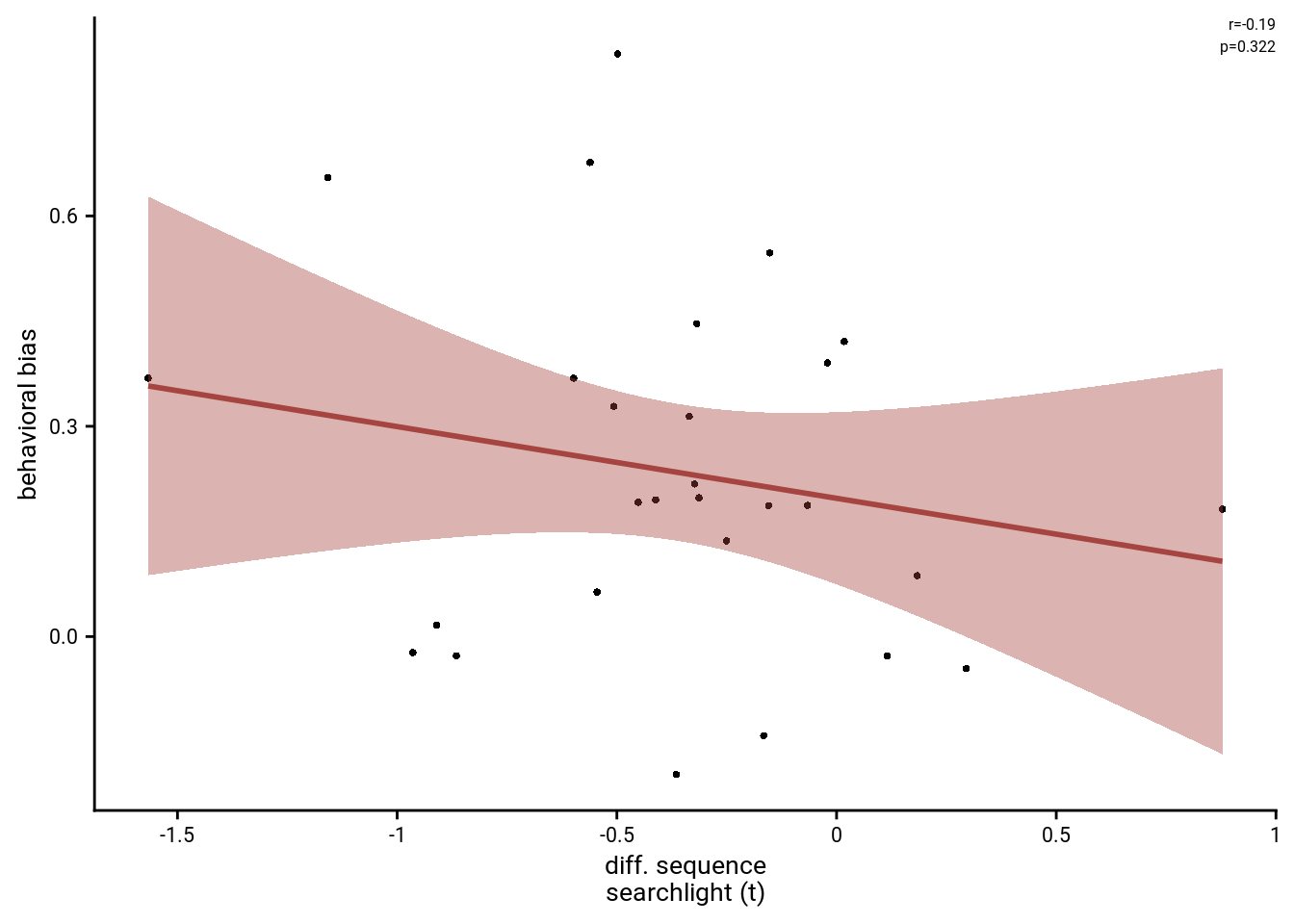
# save source data
source_dat <-ggplot_build(f8e)$data[[1]]
readr::write_tsv(source_dat %>% select(x,y),
file = file.path(dirs$source_dat_dir, "f8e.txt"))Correlation with same-sequence searchlight effect
Next, we look for a correlation with the same-sequence searchlight effect. Again, we might expect to see a negative correlation: Participants with a stronger representation of the within-sequence relationships might be less biased in their construction by the overall structure.
# load the p-values from same-sequence searchlight (SVC corrected)
p_fn <- file.path(dirs$data4analysis, "searchlight_results", "same_day_vir_time",
"same_day_vir_time_randomise_svc_fwhm3_tfce_corrp_tstat1.nii.gz")
p_nii <- readNIfTI2(p_fn)
# load the 4D image with searchlight t-values for each participant
tvals_fn <- file.path(dirs$data4analysis, "searchlight_results", "same_day_vir_time",
"same_day_vir_time_4d_smooth_fwhm3.nii.gz")
t_nii <- readNIfTI2(tvals_fn)
# find the coordinates of peak voxel
coords<-which(p_nii ==max(p_nii))
# store the searchlight t-value for each subject at this voxel
fit_beh_bias <- fit_beh_bias %>% add_column(srchlght_t=NA)
for (i in 1:28){
curr_nii <- t_nii[,,,i]
fit_beh_bias$srchlght_t[i] <- mean(curr_nii[cbind(coords)])
}
# correlate the same-sequence searchlight effect with the behavioral bias
stats <- tidy(cor.test(fit_beh_bias$beta_rel_time_other_events, fit_beh_bias$srchlght_t,
method="spearman"))
# print results
huxtable(stats) %>% theme_article() | estimate | statistic | p.value | method | alternative |
|---|---|---|---|---|
| -0.526 | 5.58e+03 | 0.00456 | Spearman's rank correlation rho | two.sided |
Spearman correlation of within-sequence searchlight effect in aHPC and behavioral generalization bias: r=-0.53, p=0.005
Indeed, we observe a significant correlation. Let’s make a plot to visualize it.
# scatterplot
f8f <- ggplot(fit_beh_bias, aes(x=srchlght_t, y=beta_rel_time_other_events))+
geom_point(size = 1, shape = 16) +
geom_smooth(method='lm', formula= y~x,
colour=unname(aHPC_colors["within_main"]),
fill=unname(aHPC_colors["within_main"]),
size=1)+
scale_x_continuous(labels = c(-0.5, 0, 0.5, 1, 1.5)) +
xlab("same sequence\nsearchlight (t)") +
ylab("behavioral bias") +
annotate("text", x=Inf, y=Inf, hjust=1,vjust=1,
size = 6/.pt, family = font2use,
label=sprintf("r=%.2f\np=%.3f",
round(stats$estimate,2), round(stats$p.value, 3))) +
theme_cowplot() +
theme(text = element_text(size=10, family=font2use),
axis.text = element_text(size=8),
legend.text=element_text(size=8),
legend.title=element_text(size=8),
legend.position = "none")
f8f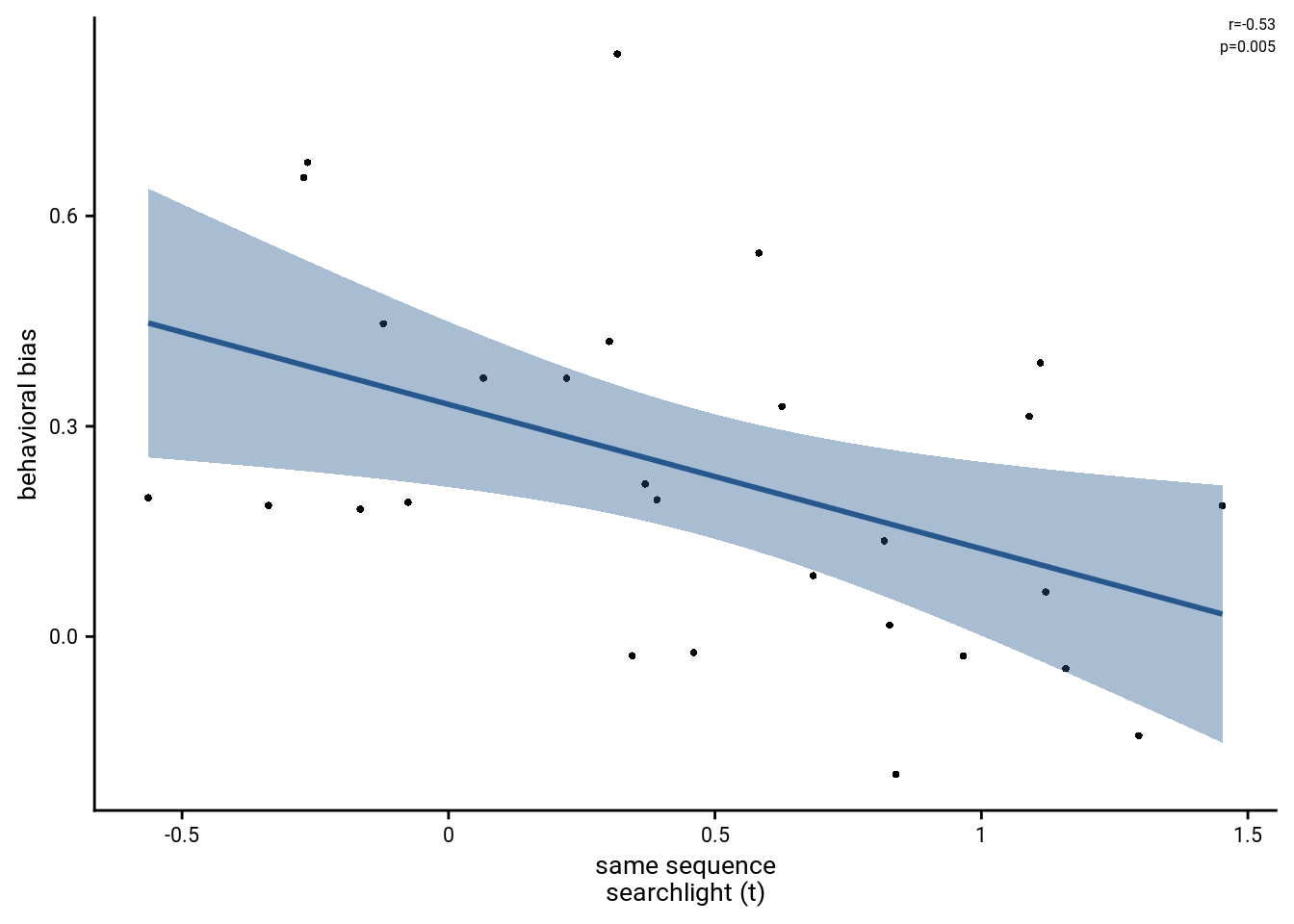
# save source data
source_dat <-ggplot_build(f8f)$data[[1]]
readr::write_tsv(source_dat %>% select(x,y),
file = file.path(dirs$source_dat_dir, "f8f.txt"))We are now ready to compose figure 8.
layout = "
ACDE
BCDF"
f8 <- plot_spacer() + f8b + f8c + f8d + f8e + f8f +
plot_layout(design = layout, guides = "keep") &
theme(text = element_text(size=10, family=font2use),
axis.text = element_text(size=8),
legend.text=element_text(size=8),
legend.title=element_text(size=8),
legend.position = "none"
) &
plot_annotation(theme = theme(plot.margin = margin(t=0, r=0, b=0, l=-5, unit="pt")),
tag_levels = list(c('B', 'C', 'D', 'E', 'F', 'G', 'H', 'I', 'J')))
# save as png and pdf and print to screen
fn <- here("figures", "f8")
ggsave(paste0(fn, ".pdf"), plot=f8, units = "cm",
width = 18, height = 10, dpi = "retina", device = cairo_pdf)
ggsave(paste0(fn, ".png"), plot=f8, units = "cm",
width = 18, height = 10, dpi = "retina", device = "png")
Figure 8. Structural knowledge biases construction of event times. A. The generalization bias quantifies the influence of structural knowledge on the construction of individual event times. For each event, the mean time of events at the same sequence position in the other sequences was calculated to test whether event times were biased towards the relative time of other events. B. The scatterplot illustrates the generalization bias for an example participant. Each circle corresponds to one event and the regression line highlights the relationship between the relative time of other events and the errors in constructed event times. The example participant was chosen to have a median-strength generalization bias. See Supplemental Figure 10 for the entire sample. Correlation coefficient is based on Pearson correlation. C. The relative time of events from other sequences predicted signed event time construction errors as measured in the timeline task. Positive values indicate that when other events took place late relative to a specific event, the time of that event was estimated to be later than when other events were relatively early. Circles show individual participant Z-values from participant-specific linear models (B); boxplot shows median and upper/lower quartile along with whiskers extending to most extreme data point within 1.5 interquartile ranges above/below the upper/lower quartile; black circle with error bars corresponds to mean±S.E.M.; distribution shows probability density function of data points. D. The generalization bias in event time construction through structural knowledge was replicated in an independent sample (n=46) based on Montijn et al.66. Data shown as in B. E. The behavioral generalization bias (regression coefficients from summary statistics approach) did not correlate significantly with the across-sequence generalization effect in the anterior hippocampus (searchlight peak voxel t-values). F. We observed a significant negative correlation between the same-sequence searchlight effect (peak voxel t-values) and the behavioral generalization bias (regression coefficients from summary statistics approach), suggesting that participants with strong hippocampal representations of the temporal relations between events from the same sequence were less biased by structural knowledge in their construction of event times. Statistics in E and F are based on Spearman correlation.
8.13 Mixed Model Summaries
Supplemental Figure
Make supplemental mixed model figure.
layout = "
ABCDEF
GHIJKL
MNOPQR"
sfigmm_a <- sfigmm_a + ggtitle("remembered times: all time metrics")
sfigmm_c <- sfigmm_c + ggtitle("aHPC same seq.: virtual time")
sfigmm_e <- sfigmm_e + ggtitle("aHPC same seq.: all time metrics")
sfigmm_g <- sfigmm_g + ggtitle("aHPC different seq.: virtual time")
sfigmm_i <- sfigmm_i + ggtitle("aHPC: interaction virtual time & seq.")
sfigmm_k <- sfigmm_k + ggtitle("alEC all events: virtual time")
sfigmm_m <- sfigmm_m + ggtitle("searchlight peak different seq.: virtual time")
sfigmm_o <- sfigmm_o + ggtitle("generalization bias (fMRI sample)")
sfigmm_q <- sfigmm_q + ggtitle("generalization bias (replication sample)")
sfigmm <- sfigmm_a +
sfigmm_b +
sfigmm_c +
sfigmm_d +
sfigmm_e +
sfigmm_f +
sfigmm_g +
sfigmm_h +
sfigmm_i +
sfigmm_j +
sfigmm_k +
sfigmm_l +
sfigmm_m +
sfigmm_n +
sfigmm_o +
sfigmm_p +
sfigmm_q +
sfigmm_r +
plot_layout(design = layout, guides = "collect") &
theme(text = element_text(size=10, family=font2use),
axis.title = element_blank(),
axis.text = element_text(size=8),
legend.text=element_text(size=8),
legend.title=element_text(size=8),
legend.position = "bottom",
legend.justification = 0,
legend.spacing.x = unit(-0.1, 'cm'),
legend.margin=margin(t = 0, r = 0.1, l = 0, b = 0, unit='cm'),
plot.title = element_text(size=8, family=font2use, hjust = 0, vjust = 1, margin = margin(t=0.2, r=0, b=0, l=0, unit = "cm")),
plot.title.position = "plot",
plot.tag.position = c(0, 1),
plot.tag = element_text(hjust = 0, vjust = 0)
) &
plot_annotation(tag_levels = "A")
# save as png and pdf and print to screen
fn <- here("figures", "sf04")
ggsave(paste0(fn, ".pdf"), plot=sfigmm, units = "cm",
width = 17.4, height = 18, dpi = "retina", device = cairo_pdf)
ggsave(paste0(fn, ".png"), plot=sfigmm, units = "cm",
width = 17.4, height = 18, dpi = "retina", device = "png")
Supplemental Figure 4. Mixed model results. Dot plots show parameter estimates and 95% CIs for fixed effects of mixed model analyses. Line plots show estimated marginal means. A, B. Remembered times in the time line task are predicted by virtual event times with order and real time in the model (c.f. Figure 2B). C, D. Temporal distances in virtual time explain representational change in the anterior hippocampus (aHPC) for same-sequence events (c.f. Figure 4B). E, F. Temporal distances in virtual time explain representational change in the aHPC for same-sequence events when competing for variance with temporal distances based on order and real time (c.f. Figure 4D). G, H. Temporal distances in virtual time explain representational change in the aHPC for different-sequence events (c.f. Figure 5A). I, J. There was a significant interaction of virtual temporal distances and sequence membership characterized by a differential relationship between temporal distances and aHPC representational change for event pairs from the same sequence or from different sequences (c.f. Figure 5A). K, L. Virtual temporal distances explain representational change in the anterior-lateral entorhinal cortex (alEC) when collapsing across all event pairs (c.f. Figure 6B). M, N. In the aHPC peak cluster of the same-sequence searchlight analysis, virtual temporal distances were siginificantly related to representational change for events from different sequences (c.f. Figure 7B). O-R. The relative time of events from other sequences predicted signed event time construction errors as measured in the timeline task (c.f. Figure 8CD) in the main fMRI sample (O, P) and in the independent replication sample (Q, R).
Supplemental Tables
Write and save the word document with the supplemental tables.
# make a list of the supplemental tables we want to write to file
stables <- list(stable_lme_memtime_time_metrics, #1
stable_lme_aHPC_virtime_same_seq, #2
stable_lme_aHPC_virtime_same_seq_first_last, #3
stable_lme_aHPC_virtime_same_seq_time_metrics, #4
stable_lme_aHPC_virtime_diff_seq, #5
stable_lme_aHPC_virtime_diff_seq_time_metrics, #6
stable_lme_aHPC_virtime_same_vs_diff_seq, #7
stable_lme_aHPC_virtime_same_vs_diff_seq_all_interactions, #8
stable_lme_alEC_virtime_all_events, #9
stable_lme_alEC_virtime_all_comps_time_metrics, #10
stable_lme_virtime_aHPC_vs_alEC, #11
stable_srchlght_same_seq, #12
stable_lme_same_seq_cluster_virtime_diff_seq, #13
stable_srchlght_diff_seq, #14
stable_srchlght_interaction, #15
stable_lme_beh_gen_bias, # 16
stable_lme_beh_gen_bias_replication) #17
# loop over tables and write to file
for (i in 1:length(stables)){
# run auto-numbering to find table number and define table heading
f_par <- officer::fpar(officer::run_autonum(seq_id = "tab",
pre_label = "Supplemental Table ",
post_label = ""))
# add table heading and table to the document
stables_docx <- stables_docx %>%
officer::body_add_fpar(f_par, style = "heading 2", pos = "after") %>% # table heading
flextable::body_add_flextable(stables[[i]], align = "left") # table
# page break if not the last table
if (i<length(stables)){
stables_docx <- stables_docx %>%
officer::body_add_break(pos = "after") # page break
}
}
# save the document
print(stables_docx, target = here("virtem_code", "docs", "supplemental_tables.docx"))8.13.1 Source data
Let’s also put all the source data into a zipped folder.
zip::zip(zipfile = file.path(dirs$source_dat_dir, "SourceData.zip"),
files = dir(dirs$source_dat_dir, full.names = TRUE),
mode = "cherry-pick")